Example #3

Introduction

Look into Intra Class Correlation (ICC)

What proportion of variability (variance) in the model is due to cluster effects

Example #3

require(flexplot)

Loading required package: flexplot

require(lme4)

Loading required package: lme4

Loading required package: Matrix

require(dplyr)

Loading required package: dplyr

Attaching package: 'dplyr'

The following objects are masked from 'package:stats':

    filter, lag

The following objects are masked from 'package:base':

    intersect, setdiff, setequal, union

#require(ggplot2)

Fit a baseline and compute ICC

data(math)
baseline <- lmer(MathAch~1 + (1|School), data=math) 
# ICC is var(school)/ ( var(school) + var(person) ) 
# e.g. when school and person vars are equal ICC is 0.5
# Increasing person var relative to school pushes toward 1 
# ICC runs 0 to 1
# ICC = 0 means perfectly independant 
# rising ICC towards 1 (or 100%) is towards non-independant
# This function extracts the necessary variances from the mixed model and computes ICC.
# Digging in the icc() function one can see it uses lme4 function VarrCorr to get variances.
#
# VarCorr {lme4} Extract Variance and Correlation Components
# This function calculates the estimated variances, standard deviations, and correlations 
# between the random-effects terms in a mixed-effects model, of class merMod (linear, 
# generalized or nonlinear). The within-group error variance and standard deviation are also # calculated.
#
# Digging: In this case try, 
# str(as.data.frame(VarCorr(baseline))
# grp  : chr  "School" "Residual"
# ..
# vcov : num  8.61 39.15
# 
# ICC is ~ 8.61 / (8.61 + 39.15) = 0.1802764
# vcov is "variances or covariances"
# Using MathAch var by school from model fit
# calculating directly, gives  different numbers
# grp_school <- math %>% group_by(School) %>% summarise(mean_MathAch = mean(MathAch)) 
# var(grp_school$mean_MathAch) 
# 9.71975
# var(math$MathAch)
# 47.31026
# 
# so, perhaps ICC in this case is better expressed as..understood by me as...
# from the model fit
# var(MathAch by school)/ ( var(MathAch by school) + var(MathAch disregarding School) ) 

icc(baseline) 

$icc
[1] 0.1803518

$design.effect
[1] 8.918571

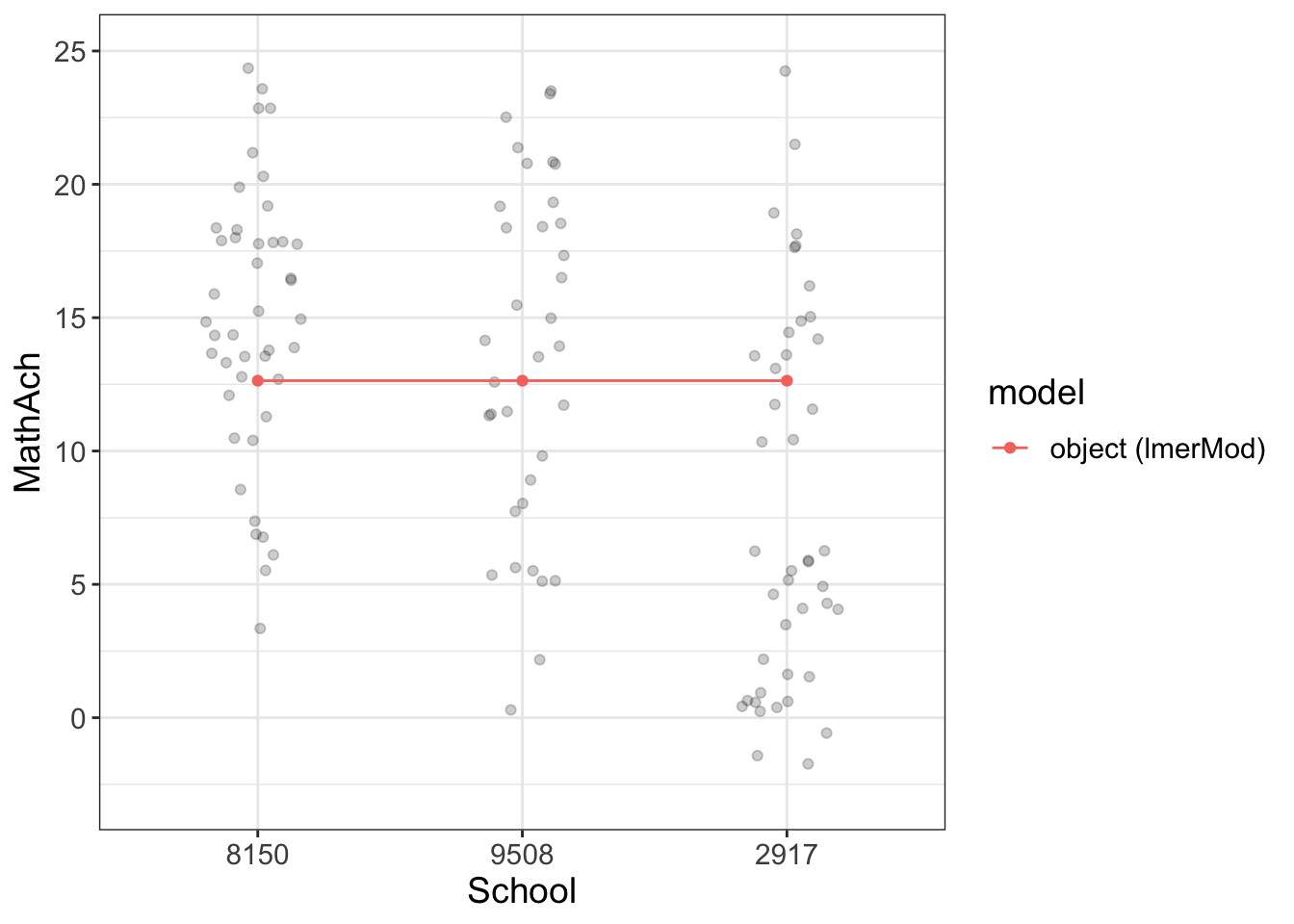
visualize(baseline, plot="model")

Coordinate system already present. Adding new coordinate system, which will
replace the existing one.

Comments

• 18% cluster effects
• my plot doesn’t show the random effects despite the model being identical to DFs

fixed_slopes <- lmer(MathAch~SES + (1|School), data=math)
visualize(fixed_slopes, plot="model")

random_slopes <- lmer(MathAch~SES + (SES|School), data=math)
visualize(random_slopes, plot="model")

# see 8 schools, 2 at a time 
compare.fits(MathAch~SES | School, data=math, fixed_slopes, random_slopes, clusters = 2)

compare.fits(MathAch~SES | School, data=math, fixed_slopes, random_slopes, clusters = 2)

compare.fits(MathAch~SES | School, data=math, fixed_slopes, random_slopes, clusters = 2)

compare.fits(MathAch~SES | School, data=math, fixed_slopes, random_slopes, clusters = 2)

# 
model.comparison(fixed_slopes, baseline)

refitting model(s) with ML (instead of REML)

$statistics
                  aic      bic  bayes.factor      p
fixed_slopes 46653.17 46680.69 3.045609e+100 <2e-16
baseline     47122.79 47143.43  0.000000e+00       

$predicted_differences
   0%   25%   50%   75%  100% 
0.000 0.532 1.095 1.825 8.917 

$r_squared_change
   Residual (Intercept) 
  0.0539978   0.4464638 

model.comparison(random_slopes, baseline)

refitting model(s) with ML (instead of REML)

$statistics
                   aic      bic bayes.factor      p
random_slopes 46652.40 46693.68 4.605423e+97 <2e-16
baseline      47122.79 47143.43 0.000000e+00       

$predicted_differences
   0%   25%   50%   75%  100% 
0.000 0.514 1.071 1.802 8.991 

$r_squared_change
   Residual (Intercept) 
 0.05921519  0.43943350 

model.comparison(fixed_slopes, random_slopes)

refitting model(s) with ML (instead of REML)

$statistics
                   aic      bic bayes.factor     p
fixed_slopes  46653.17 46680.69      661.309 0.104
random_slopes 46652.40 46693.68        0.002      

$predicted_differences
   0%   25%   50%   75%  100% 
0.000 0.024 0.070 0.162 2.008 

$r_squared_change
    Residual  (Intercept) 
-0.005545779  0.012541409 

# fixed_slopes is probably better
summary(fixed_slopes)

Linear mixed model fit by REML ['lmerMod']
Formula: MathAch ~ SES + (1 | School)
   Data: math

REML criterion at convergence: 46645.2

Scaled residuals: 
     Min       1Q   Median       3Q      Max 
-3.12607 -0.72720  0.02188  0.75772  2.91912 

Random effects:
 Groups   Name        Variance Std.Dev.
 School   (Intercept)  4.768   2.184   
 Residual             37.034   6.086   
Number of obs: 7185, groups:  School, 160

Fixed effects:
            Estimate Std. Error t value
(Intercept)  12.6575     0.1880   67.33
SES           2.3902     0.1057   22.61

Correlation of Fixed Effects:
    (Intr)
SES 0.003 

# genrally categorical vars are fixed effects
with_minority =  lmer(MathAch~SES + Minority + (SES|School), data=math)
compare.fits(MathAch~SES | Minority + School, data=math, with_minority, fixed_slopes)

model.comparison(with_minority, fixed_slopes)

refitting model(s) with ML (instead of REML)

$statistics
                   aic      bic bayes.factor      p
with_minority 46457.03 46505.19 1.286257e+38 <2e-16
fixed_slopes  46653.17 46680.69 0.000000e+00       

$predicted_differences
   0%   25%   50%   75%  100% 
0.000 0.197 0.461 0.990 3.603 

$r_squared_change
   Residual (Intercept) 
 0.02802041  0.17449215 

summary(with_minority)

Linear mixed model fit by REML ['lmerMod']
Formula: MathAch ~ SES + Minority + (SES | School)
   Data: math

REML criterion at convergence: 46443

Scaled residuals: 
    Min      1Q  Median      3Q     Max 
-3.1742 -0.7243  0.0283  0.7577  3.0047 

Random effects:
 Groups   Name        Variance Std.Dev. Corr 
 School   (Intercept)  3.9362  1.9840        
          SES          0.3187  0.5645   -0.40
 Residual             35.9967  5.9997        
Number of obs: 7185, groups:  School, 160

Fixed effects:
            Estimate Std. Error t value
(Intercept)  13.5047     0.1827   73.92
SES           2.1326     0.1156   18.44
MinorityYes  -2.9782     0.2081  -14.31

Correlation of Fixed Effects:
            (Intr) SES   
SES         -0.194       
MinorityYes -0.307  0.173

Comments

• Akaike information criterion (AIC)

• Bayesian information criterion (BIC) or Schwarz information criterion (also SIC, SBC, SBIC)

• Looking at summary(with_minority), the model parameters are pretty similar to Example #2 - the standard linear model (lm2 <- lm(MathAch ~ SES + Minority, data = math))

# software library update
# estimates() has become available

# explain of dessign.effect - artificail infaltion 
estimates(with_minority)

refitting model(s) with ML (instead of REML)

Fixed Effects: 
(Intercept)         SES MinorityYes 
  13.504724    2.132604   -2.978157 


Random Effects: 
 Groups   Name        Std.Dev. Corr  
 School   (Intercept) 1.9840         
          SES         0.5645   -0.400
 Residual             5.9997         


ICC and Design Effect: 
          icc design.effect 
    0.1803518     8.9185709 


R Squared: 

   Residual (Intercept) 
 0.08050517  0.54305152