Example #1

Introduction

Some examples of using “flexplot” and “lmer” based on the excellent explanations from Dustin Fife (Video Link). Modified with tidyverse packages and plots (ggplot) to enable additional data understanding. My annotations and observations in line with code. Wrapped up in a Quarto package.

Example #1

require(flexplot)

Loading required package: flexplot

require(lme4)

Loading required package: lme4

Loading required package: Matrix

require(dplyr)

Loading required package: dplyr


Attaching package: 'dplyr'

The following objects are masked from 'package:stats':

    filter, lag

The following objects are masked from 'package:base':

    intersect, setdiff, setequal, union

Data about alcohol use in teenagers is distributed with flexplot.

data(alcuse)
# see some data
head(alcuse, 10)

   ID AGE COA MALE AGE_14   ALCUSE      PEER      CPEER  CCOA
1   1  14   1    0      0 1.732051 1.2649111  0.2469111 0.549
2   1  15   1    0      1 2.000000 1.2649111  0.2469111 0.549
3   1  16   1    0      2 2.000000 1.2649111  0.2469111 0.549
4   2  14   1    1      0 0.000000 0.8944272 -0.1235728 0.549
5   2  15   1    1      1 0.000000 0.8944272 -0.1235728 0.549
6   2  16   1    1      2 1.000000 0.8944272 -0.1235728 0.549
7   3  14   1    1      0 1.000000 0.8944272 -0.1235728 0.549
8   3  15   1    1      1 2.000000 0.8944272 -0.1235728 0.549
9   3  16   1    1      2 3.316625 0.8944272 -0.1235728 0.549
10  4  14   1    1      0 0.000000 1.7888544  0.7708544 0.549

# rows
paste0(nrow(alcuse), " rows of data.")

[1] "246 rows of data."

# number of groups and data points
alcuse_sum <- alcuse %>% group_by(ID) %>% 
  summarise(mean = mean(ALCUSE), n_ALCUSE = n()) %>% print(n = 20)

# A tibble: 82 × 3
      ID  mean n_ALCUSE
   <int> <dbl>    <int>
 1     1 1.91         3
 2     2 0.333        3
 3     3 2.11         3
 4     4 1.24         3
 5     5 0            3
 6     6 3.05         3
 7     7 1.73         3
 8     8 0            3
 9     9 1.49         3
10    10 1            3
11    11 1.05         3
12    12 0.911        3
13    13 0.667        3
14    14 3.09         3
15    15 2.14         3
16    16 1.28         3
17    17 0.333        3
18    18 1.58         3
19    19 0            3
20    20 2.64         3
# ℹ 62 more rows

# number of groups check 
# 3 measures for each ID
nrow(filter(alcuse_sum, n_ALCUSE == 3))

[1] 82

Comments

There are 3 measurements of ALCUSE for each of 82 IDs.

Probably a boxplot is more useful to get a feel for the data (TODO)

summary(alcuse)

       ID            AGE          COA              MALE            AGE_14 
 Min.   : 1.0   Min.   :14   Min.   :0.0000   Min.   :0.0000   Min.   :0  
 1st Qu.:21.0   1st Qu.:14   1st Qu.:0.0000   1st Qu.:0.0000   1st Qu.:0  
 Median :41.5   Median :15   Median :0.0000   Median :1.0000   Median :1  
 Mean   :41.5   Mean   :15   Mean   :0.4512   Mean   :0.5122   Mean   :1  
 3rd Qu.:62.0   3rd Qu.:16   3rd Qu.:1.0000   3rd Qu.:1.0000   3rd Qu.:2  
 Max.   :82.0   Max.   :16   Max.   :1.0000   Max.   :1.0000   Max.   :2  
     ALCUSE           PEER            CPEER                 CCOA           
 Min.   :0.000   Min.   :0.0000   Min.   :-1.0180000   Min.   :-0.4510000  
 1st Qu.:0.000   1st Qu.:0.0000   1st Qu.:-1.0180000   1st Qu.:-0.4510000  
 Median :1.000   Median :0.8944   Median :-0.1235728   Median :-0.4510000  
 Mean   :0.922   Mean   :1.0176   Mean   :-0.0004405   Mean   : 0.0002195  
 3rd Qu.:1.732   3rd Qu.:1.5492   3rd Qu.: 0.5311934   3rd Qu.: 0.5490000  
 Max.   :3.606   Max.   :2.5298   Max.   : 1.5118221   Max.   : 0.5490000

Model of alcohol use. No predictors.

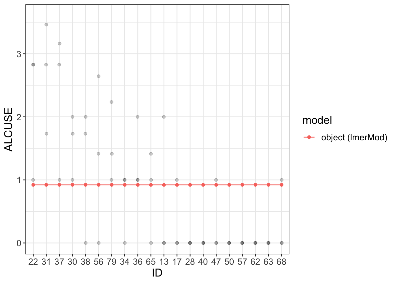
# Fixed effect + random effects
# Fixed effect: ~1 is gammma 00
# Random effects: 1 is Uij for ID 
mod = lmer(ALCUSE~1 + (1|ID), data=alcuse)
visualize(mod, plot = "model", sample = 20)

Coordinate system already present. Adding new coordinate system, which will
replace the existing one.

summary(mod)

Linear mixed model fit by REML ['lmerMod']
Formula: ALCUSE ~ 1 + (1 | ID)
   Data: alcuse

REML criterion at convergence: 673

Scaled residuals: 
    Min      1Q  Median      3Q     Max 
-1.8892 -0.3079 -0.3029  0.6111  2.8562 

Random effects:
 Groups   Name        Variance Std.Dev.
 ID       (Intercept) 0.5731   0.7571  
 Residual             0.5617   0.7495  
Number of obs: 246, groups:  ID, 82

Fixed effects:
            Estimate Std. Error t value
(Intercept)   0.9220     0.0963   9.574

Comments

Dustin’s model visualize() plot does not look like this one despite the code being identical.

The visualize function defaults to 3 random IDs (?). I change it (with sample = n)

Looks like Dustin’s data is normalized to 1

Dustin gets Fixed Effect and Random Effects plotted. I just get: object (lmerMod).

However the summary(mod) is identical to Dustin’s.

# always useful to look this way
summary(mod)

Linear mixed model fit by REML ['lmerMod']
Formula: ALCUSE ~ 1 + (1 | ID)
   Data: alcuse

REML criterion at convergence: 673

Scaled residuals: 
    Min      1Q  Median      3Q     Max 
-1.8892 -0.3079 -0.3029  0.6111  2.8562 

Random effects:
 Groups   Name        Variance Std.Dev.
 ID       (Intercept) 0.5731   0.7571  
 Residual             0.5617   0.7495  
Number of obs: 246, groups:  ID, 82

Fixed effects:
            Estimate Std. Error t value
(Intercept)   0.9220     0.0963   9.574

Comments

The model Intercept 0.9220 is simply the mean of the ALCUSE variable

signif(mean(alcuse$ALCUSE),4)

[1] 0.922

Random intercepts model

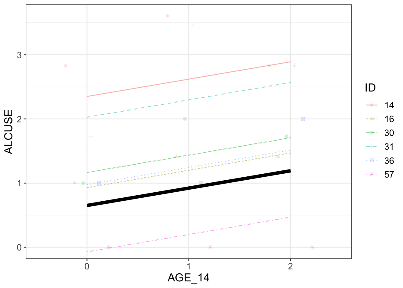
# random intercepts using AGE_14 as predictor for fixed IDs
# AGE_14 predictor (fixed gradients)
# (1|ID) tells intercepts may vary (random intercepts)
rand.i <- lmer(ALCUSE~1 + AGE_14 + (1|ID), data = alcuse)
# by default 3 IDs are plotted
sample_n <- 6
# if all groups are plotted, one gets funny comments :)
# very nice humour
# sample_n <- 82
visualize(rand.i, plot = "model", sample=sample_n)

summary(rand.i)

Linear mixed model fit by REML ['lmerMod']
Formula: ALCUSE ~ 1 + AGE_14 + (1 | ID)
   Data: alcuse

REML criterion at convergence: 654.1

Scaled residuals: 
     Min       1Q   Median       3Q      Max 
-2.19816 -0.66940  0.03001  0.44728  2.66167 

Random effects:
 Groups   Name        Variance Std.Dev.
 ID       (Intercept) 0.5966   0.7724  
 Residual             0.4915   0.7011  
Number of obs: 246, groups:  ID, 82

Fixed effects:
            Estimate Std. Error t value
(Intercept)  0.65130    0.11077   5.880
AGE_14       0.27065    0.05474   4.944

Correlation of Fixed Effects:
       (Intr)
AGE_14 -0.494

Comments

Fixed effect (Intercept) means 0.65130 drinks on average at age 14.

For subsequent years the number of drinks increases on average by 0.27065.

Random slopes (gradient) model

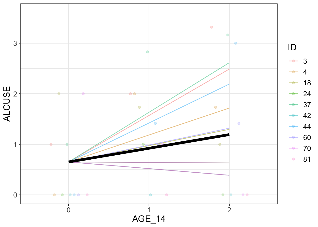
# unrealistic 
# -1 means intercept is fixed
# need to consider the level 1 and 2 models to specify the syntax correctly
rand.s <- lmer(ALCUSE~1 + AGE_14 + (-1 + AGE_14|ID), data = alcuse)
sample_n <- 10
visualize(rand.s, plot = "model", sample=sample_n)

It looks like you're trying to plot more than 6 colors/lines/symbols.
I gotta give it to you...you're ambitious. Alas, I can't do that, so I'm removing the colors/lines/symbols.
 I hope we can still be friends.

summary(rand.s)

Linear mixed model fit by REML ['lmerMod']
Formula: ALCUSE ~ 1 + AGE_14 + (-1 + AGE_14 | ID)
   Data: alcuse

REML criterion at convergence: 697.6

Scaled residuals: 
    Min      1Q  Median      3Q     Max 
-1.5231 -0.7636 -0.4583  0.4239  3.1493 

Random effects:
 Groups   Name   Variance Std.Dev.
 ID       AGE_14 0.2225   0.4717  
 Residual        0.7163   0.8463  
Number of obs: 246, groups:  ID, 82

Fixed effects:
            Estimate Std. Error t value
(Intercept)  0.65130    0.08532   7.634
AGE_14       0.27065    0.08415   3.216

Correlation of Fixed Effects:
       (Intr)
AGE_14 -0.608

Comments

Despite the warning, visualize seems to do the job with 10 samples

Random slopes and intercepts model

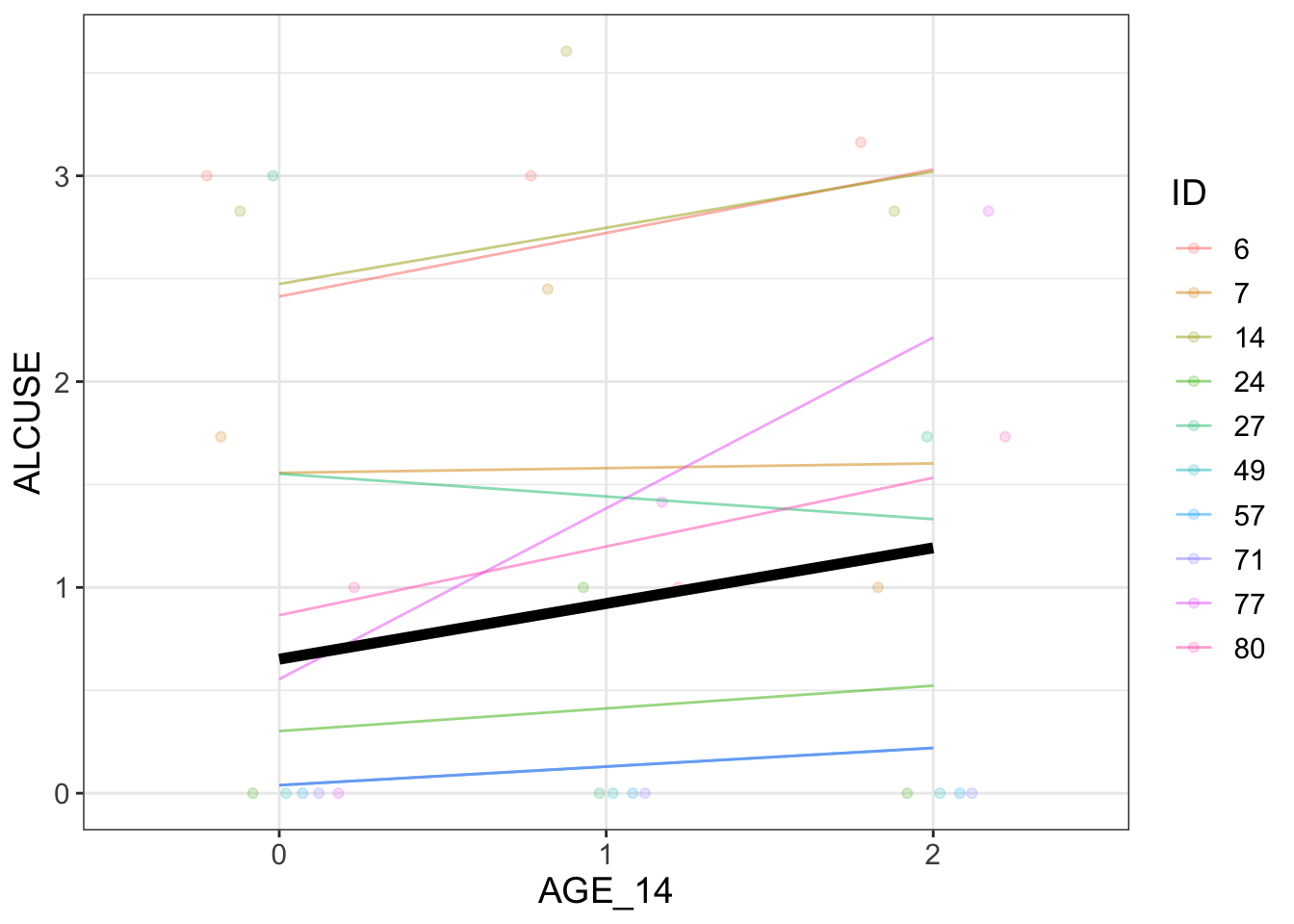
# probably what we want
# need to consider the level 1 and 2 models to specify the syntax correctly
rand.is <- lmer(ALCUSE~1 + AGE_14 + (AGE_14|ID), data = alcuse)
sample_n <- 10
visualize(rand.is, plot = "model", sample=sample_n)

It looks like you're trying to plot more than 6 colors/lines/symbols.
I gotta give it to you...you're ambitious. Alas, I can't do that, so I'm removing the colors/lines/symbols.
 I hope we can still be friends.

summary(rand.is)

Linear mixed model fit by REML ['lmerMod']
Formula: ALCUSE ~ 1 + AGE_14 + (AGE_14 | ID)
   Data: alcuse

REML criterion at convergence: 643.2

Scaled residuals: 
     Min       1Q   Median       3Q      Max 
-2.48287 -0.37933 -0.07858  0.38876  2.49284 

Random effects:
 Groups   Name        Variance Std.Dev. Corr 
 ID       (Intercept) 0.6355   0.7972        
          AGE_14      0.1552   0.3939   -0.23
 Residual             0.3373   0.5808        
Number of obs: 246, groups:  ID, 82

Fixed effects:
            Estimate Std. Error t value
(Intercept)  0.65130    0.10573   6.160
AGE_14       0.27065    0.06284   4.307

Correlation of Fixed Effects:
       (Intr)
AGE_14 -0.441