Example #4

Overview

A stripped down version of Example #1, modified to allow key parameters to be easily changed in order to look at the stability of the final results.

Tests and results:

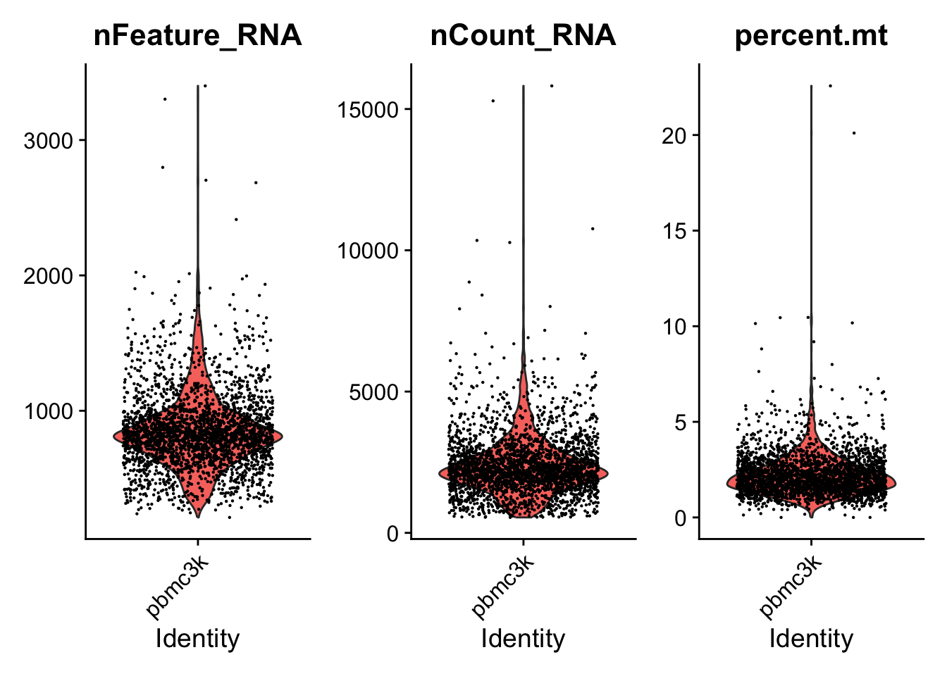
• Like Example #1, nFeature_RNA is cut at 2500

• FindClusters resolution is reset to the Example #1 default of 0.5

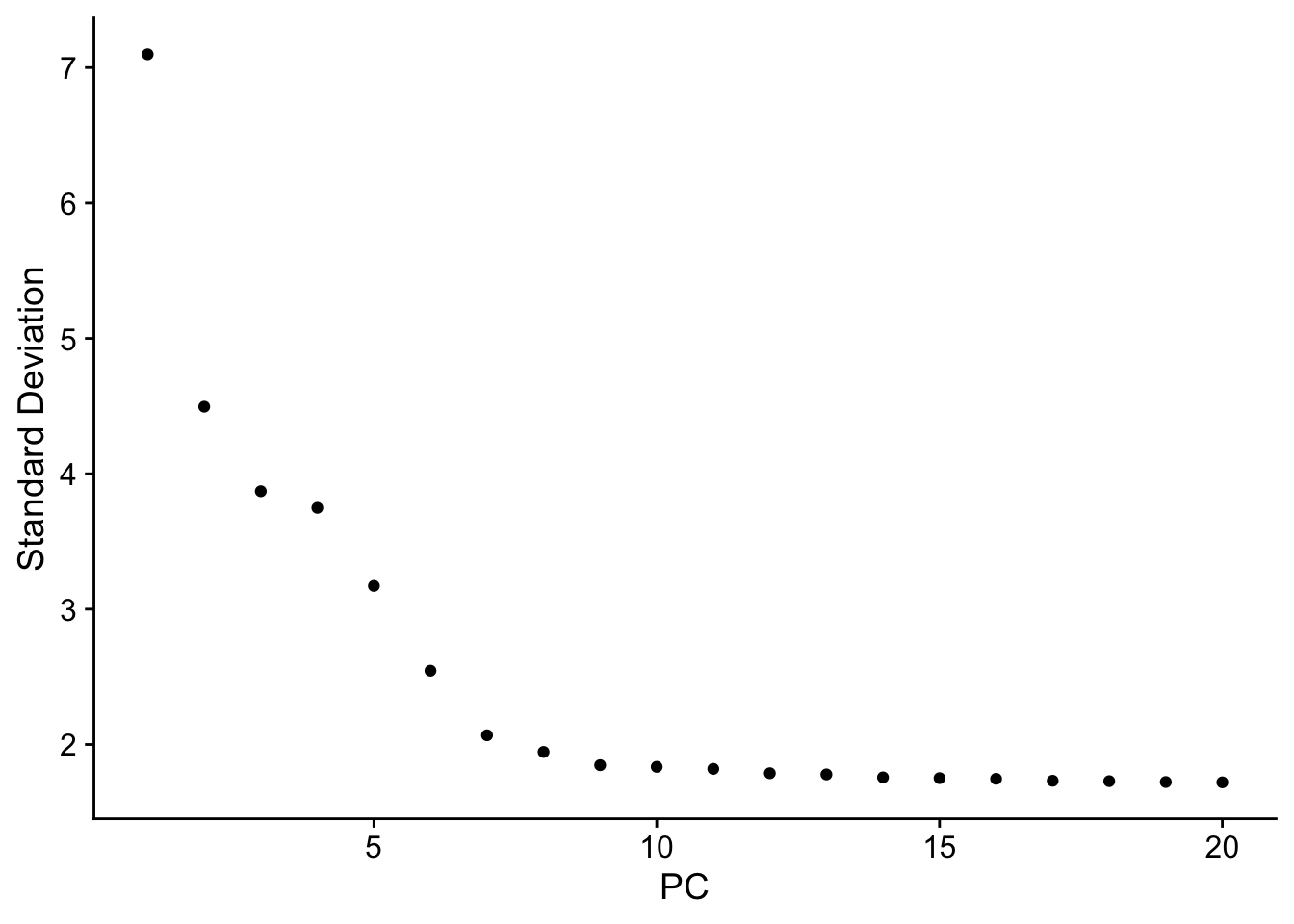
• The number of Principal Components (PCs) used in clustering is generated as a series: 2, 3, 5, 7 and is compared to 10

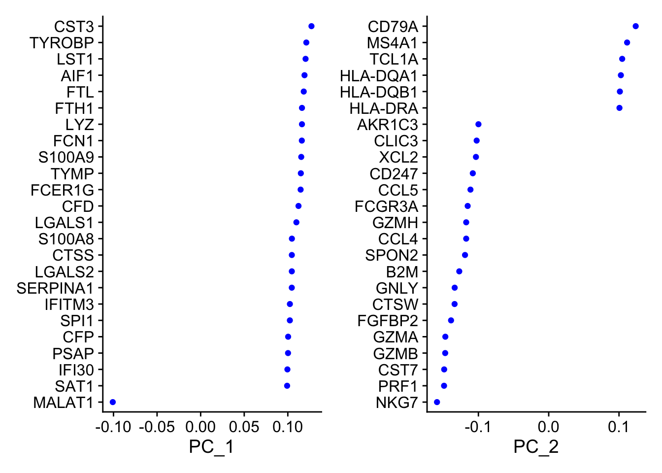
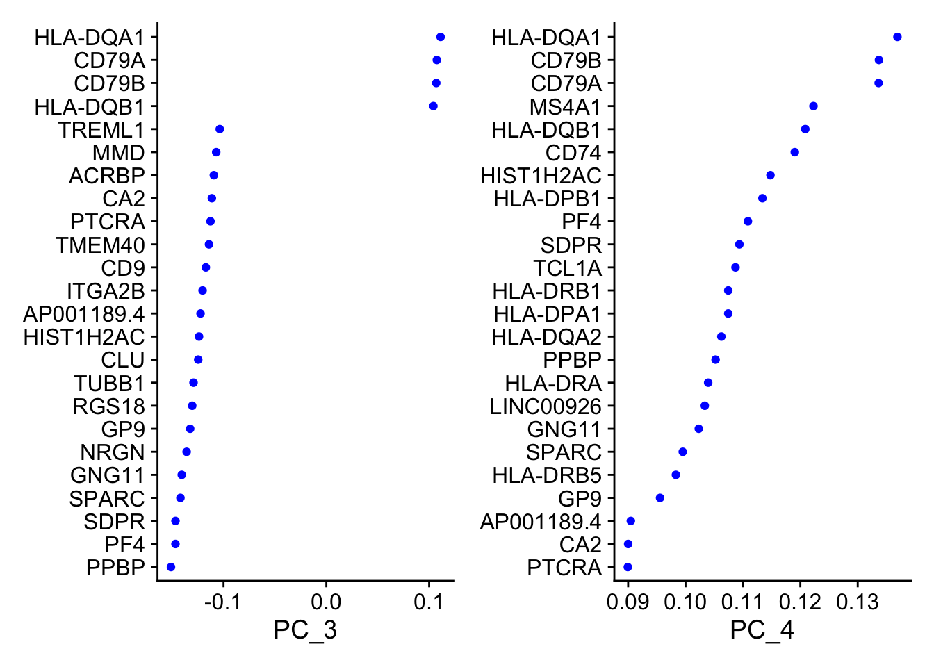
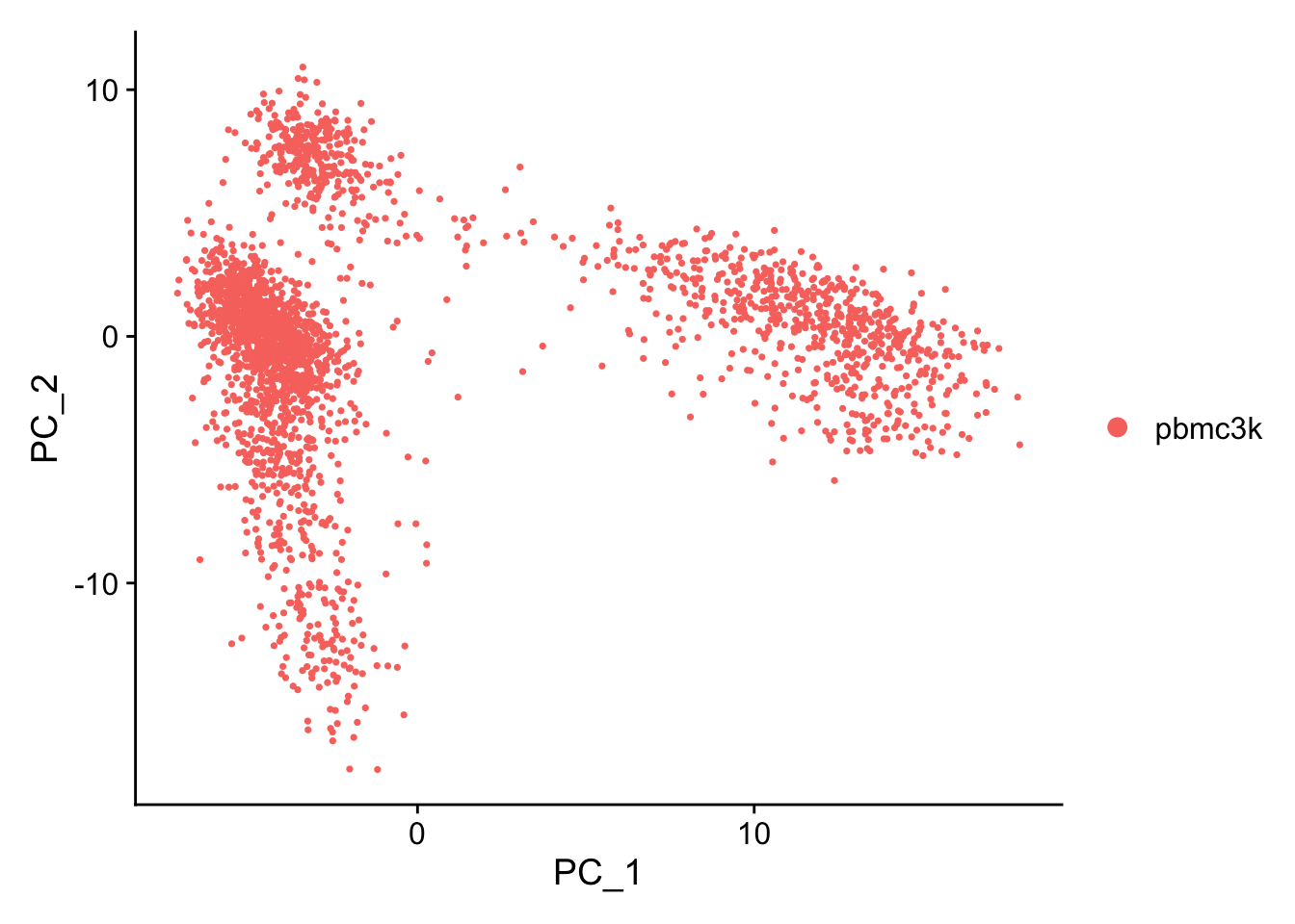
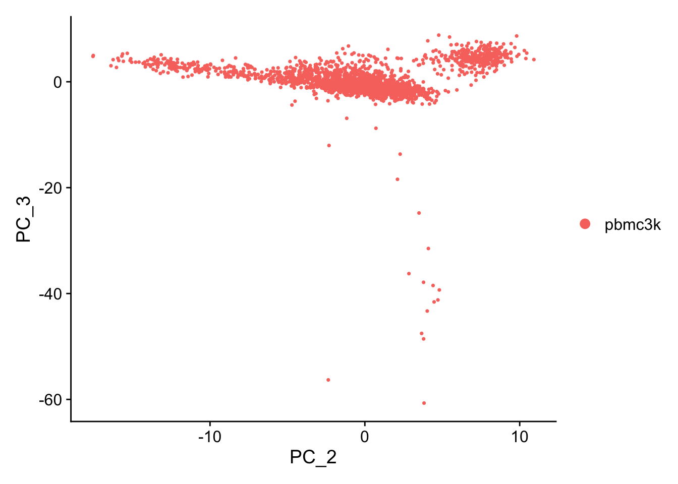
• A nice demonstration of choosing a sufficient number of PCs

Includes

Environment Load and Check

• this code section is packaged as an include for reuse across all examples
• it uses the HTML details tag directly to wrap code blocks and output as drop-down sections

Show Environment

library(patchwork)
library(dplyr)

Attaching package: 'dplyr'

The following objects are masked from 'package:stats':

    filter, lag

The following objects are masked from 'package:base':

    intersect, setdiff, setequal, union

library(Seurat)

Loading required package: SeuratObject

Loading required package: sp

'SeuratObject' was built under R 4.3.0 but the current version is
4.3.2; it is recomended that you reinstall 'SeuratObject' as the ABI
for R may have changed

Attaching package: 'SeuratObject'

The following object is masked from 'package:base':

    intersect

• Is there a typo in the message above? Application Programming Interface, API != ABI

• Rolling back to R 4.3.0 was not possible with the current version of Seurat

  • the indication was that Seurat requires a version of base Matrix that is not present in R 4.3.0

# which Seurat?
packageVersion("Seurat")

[1] '5.0.0'

# which R?
version[['version.string']]

[1] "R version 4.3.2 (2023-10-31)"

# presto was installed 
# For a (much!) faster implementation of the 
# Wilcoxon Rank Sum Test
packageVersion('presto')

[1] '1.0.0'

# check python is available via reticulate
import sys
print(sys.version.split(" ")[0])

3.12.0

# shell check
python3 -V

Python 3.12.0

# shell check
quarto -v

1.4.489

Functions

Show Functions

# Useful for code development.
# Save the object at a point and reload it into the R console 
# i.e. for developing alternative reports 
# without having to run the pipeline right from the start
# which can be slow
#
# NB: Files produced by saveRDS (or serialized to a file connection) 
# are not suitable as an interchange format between machines
# 
# For that use hdf5 or transfer data and code to reproduce the result 

saveRDS_overwrite <- function(file_path) {
  if (file.exists(file_path)) {
    file.remove(file_path)
  } 
  saveRDS(pbmc, file = file_path)
}

Process

# Verbose comments in Example #1 
# This is the Example (EG) Number identfier
# Should be changed for each example script
# Used in storing objects as files
EGN <- '_Eg4'

# read & create object
data_dir <- "./filtered_gene_bc_matrices/hg19/"
pbmc.data <- Read10X(data.dir = data_dir)
pbmc <- CreateSeuratObject(counts = pbmc.data, 
                           project = "pbmc3k", 
                           min.cells = 3, 
                           min.features = 200)

Warning: Feature names cannot have underscores ('_'), replacing with dashes
('-')

# calculate %mitochondrial
pbmc[["percent.mt"]] <- PercentageFeatureSet(pbmc, pattern = "^MT-")
# Visualize QC metrics as a violin plot
VlnPlot(pbmc, features = c("nFeature_RNA", "nCount_RNA", "percent.mt"),
        ncol = 3)

Warning: Default search for "data" layer in "RNA" assay yielded no results;
utilizing "counts" layer instead.

plot1 <- FeatureScatter(pbmc, feature1 = "nCount_RNA", feature2 = "percent.mt")
plot2 <- FeatureScatter(pbmc, feature1 = "nCount_RNA", feature2 = "nFeature_RNA")
plot1 + plot2

# apply filters and overwrite the object
# 
nFeature_RNA_Max <- 2500
# nFeature_RNA_Max <- 3000
# nFeature_RNA_Max <- 2100
# i.e. not cut
# nFeature_RNA_Max <- 4000

pbmc <- subset(pbmc, subset = nFeature_RNA > 200 & 
                 nFeature_RNA < nFeature_RNA_Max & percent.mt < 5)
# And we can see clearly the effect of filtering
plot1 <- FeatureScatter(pbmc, feature1 = "nCount_RNA", feature2 = "percent.mt")
plot2 <- FeatureScatter(pbmc, feature1 = "nCount_RNA", feature2 = "nFeature_RNA")
plot1 + plot2

# normalise 
pbmc <- NormalizeData(pbmc, normalization.method = "LogNormalize", 
                      scale.factor = 10000)

Normalizing layer: counts

# variable freatures (genes)
pbmc <- FindVariableFeatures(pbmc, selection.method = "vst", nfeatures = 2000)

Finding variable features for layer counts

n_top <- 15
top_v_genes <- head(VariableFeatures(pbmc), n_top)
top_v_genes

 [1] "PPBP"    "LYZ"     "S100A9"  "IGLL5"   "GNLY"    "FTL"     "PF4"    
 [8] "FTH1"    "GNG11"   "S100A8"  "FCER1A"  "HLA-DRA" "CD74"    "CLU"    
[15] "NKG7"   

# plot variable features with and without labels
plot1 <- VariableFeaturePlot(pbmc)
plot2 <- LabelPoints(plot = plot1, points = top_v_genes, repel = TRUE)

When using repel, set xnudge and ynudge to 0 for optimal results

plot2 

Warning: Transformation introduced infinite values in continuous x-axis

# scale all 
all.genes <- rownames(pbmc)
pbmc <- ScaleData(pbmc, features = all.genes)

Centering and scaling data matrix

# linear dim reduction
pbmc <- RunPCA(pbmc, verbose = FALSE)
n_features <- 8
print(pbmc[["pca"]], dims = 1:4, nfeatures = n_features)

PC_ 1 
Positive:  CST3, TYROBP, LST1, AIF1, FTL, FTH1, LYZ, FCN1 
Negative:  MALAT1, LTB, IL32, IL7R, CD2, B2M, ACAP1, CD27 
PC_ 2 
Positive:  CD79A, MS4A1, TCL1A, HLA-DQA1, HLA-DQB1, HLA-DRA, LINC00926, CD79B 
Negative:  NKG7, PRF1, CST7, GZMB, GZMA, FGFBP2, CTSW, GNLY 
PC_ 3 
Positive:  HLA-DQA1, CD79A, CD79B, HLA-DQB1, HLA-DPB1, HLA-DPA1, CD74, MS4A1 
Negative:  PPBP, PF4, SDPR, SPARC, GNG11, NRGN, GP9, RGS18 
PC_ 4 
Positive:  HLA-DQA1, CD79B, CD79A, MS4A1, HLA-DQB1, CD74, HIST1H2AC, HLA-DPB1 
Negative:  VIM, IL7R, S100A6, IL32, S100A8, S100A4, GIMAP7, S100A10 

# V
n_mulitplier = 3
VizDimLoadings(pbmc, dims = 1:2, 
               reduction = "pca", 
               nfeatures = n_features * n_mulitplier)

VizDimLoadings(pbmc, dims = 3:4, 
               reduction = "pca", 
               nfeatures = n_features * n_mulitplier)

# U 
# Dimplot has lots of options
DimPlot(pbmc, reduction = "pca",  dims = c(1, 2))

DimPlot(pbmc, reduction = "pca",  dims = c(2, 3))

# as in quote above, 
# ordererd cells and genes according to PCA scores 

# heatmaps 
n_cells <- 300
n_genes <- 24
# 1
DimHeatmap(pbmc, dims = 1, cells = n_cells, nfeatures = n_genes, balanced = TRUE)

# many
n_PC <- 6
plots <- DimHeatmap(pbmc, dims = 1:n_PC, cells = n_cells, 
             nfeatures = n_genes, balanced = TRUE)

# elbow plot
ElbowPlot(pbmc)

#n_pcs_chosen <- 10
# n_pcs_chosen <- 2
#n_pcs_chosen <- 3
#n_pcs_chosen <- 5
n_pcs_chosen <- 7

# clusters
# create the K-nearest neighbor (KNN) graph of cells
pbmc <- FindNeighbors(pbmc, dims = 1:n_pcs_chosen)

Computing nearest neighbor graph

Computing SNN

# define clusters according to resolution
pbmc <- FindClusters(pbmc, resolution = 0.5)

Modularity Optimizer version 1.3.0 by Ludo Waltman and Nees Jan van Eck

Number of nodes: 2638
Number of edges: 88288

Running Louvain algorithm...
Maximum modularity in 10 random starts: 0.8827
Number of communities: 10
Elapsed time: 0 seconds

#pbmc <- FindClusters(pbmc, resolution = 1.0)
#pbmc <- FindClusters(pbmc, resolution = 0.2)

# Look at cluster IDs of the first 5 cells
# In this case we have 9 levels (0 - 8)
# The structure is the relation between cell barcode and the cluster (community) 
head(Idents(pbmc), 5)

AAACATACAACCAC-1 AAACATTGAGCTAC-1 AAACATTGATCAGC-1 AAACCGTGCTTCCG-1 
               1                2                1                4 
AAACCGTGTATGCG-1 
               7 
Levels: 0 1 2 3 4 5 6 7 8 9

# Each cell that survived filtering above is represented 
length(Idents(pbmc))

[1] 2638

pbmc

An object of class Seurat 
13714 features across 2638 samples within 1 assay 
Active assay: RNA (13714 features, 2000 variable features)
 3 layers present: counts, data, scale.data
 1 dimensional reduction calculated: pca

# UMAP
pbmc <- RunUMAP(pbmc, dims = 1:n_pcs_chosen)

Warning: The default method for RunUMAP has changed from calling Python UMAP via reticulate to the R-native UWOT using the cosine metric
To use Python UMAP via reticulate, set umap.method to 'umap-learn' and metric to 'correlation'
This message will be shown once per session

16:21:48 UMAP embedding parameters a = 0.9922 b = 1.112

16:21:48 Read 2638 rows and found 7 numeric columns

16:21:48 Using Annoy for neighbor search, n_neighbors = 30

16:21:48 Building Annoy index with metric = cosine, n_trees = 50

0%   10   20   30   40   50   60   70   80   90   100%

[----|----|----|----|----|----|----|----|----|----|

**************************************************|
16:21:48 Writing NN index file to temp file /var/folders/zp/wn7hdby52ds73hv9g_dxlk380000gn/T//RtmpnNu5g6/file16aa4aac7fa1
16:21:48 Searching Annoy index using 1 thread, search_k = 3000
16:21:49 Annoy recall = 100%
16:21:50 Commencing smooth kNN distance calibration using 1 thread with target n_neighbors = 30
16:21:50 Initializing from normalized Laplacian + noise (using RSpectra)
16:21:50 Commencing optimization for 500 epochs, with 102208 positive edges
16:21:55 Optimization finished

DimPlot(pbmc, reduction = "umap")

# tSNE
pbmc <- RunTSNE(pbmc, dims = 1:n_pcs_chosen)
DimPlot(pbmc, reduction = "tsne")

# save the object 
file_path <- paste0("./seurat_object_checkpoints/pbmc_sw1",EGN,".rds")
saveRDS_overwrite(file_path)

# to restore
# pbmc <- readRDS(file_path)

# find markers for every cluster compared to all remaining cells, 
# report only the positive ones
pbmc.markers <- FindAllMarkers(pbmc, only.pos = TRUE, 
                                 min.pct = 0.25, logfc.threshold = 0.25)

Calculating cluster 0
Calculating cluster 1
Calculating cluster 2
Calculating cluster 3
Calculating cluster 4
Calculating cluster 5
Calculating cluster 6
Calculating cluster 7
Calculating cluster 8
Calculating cluster 9

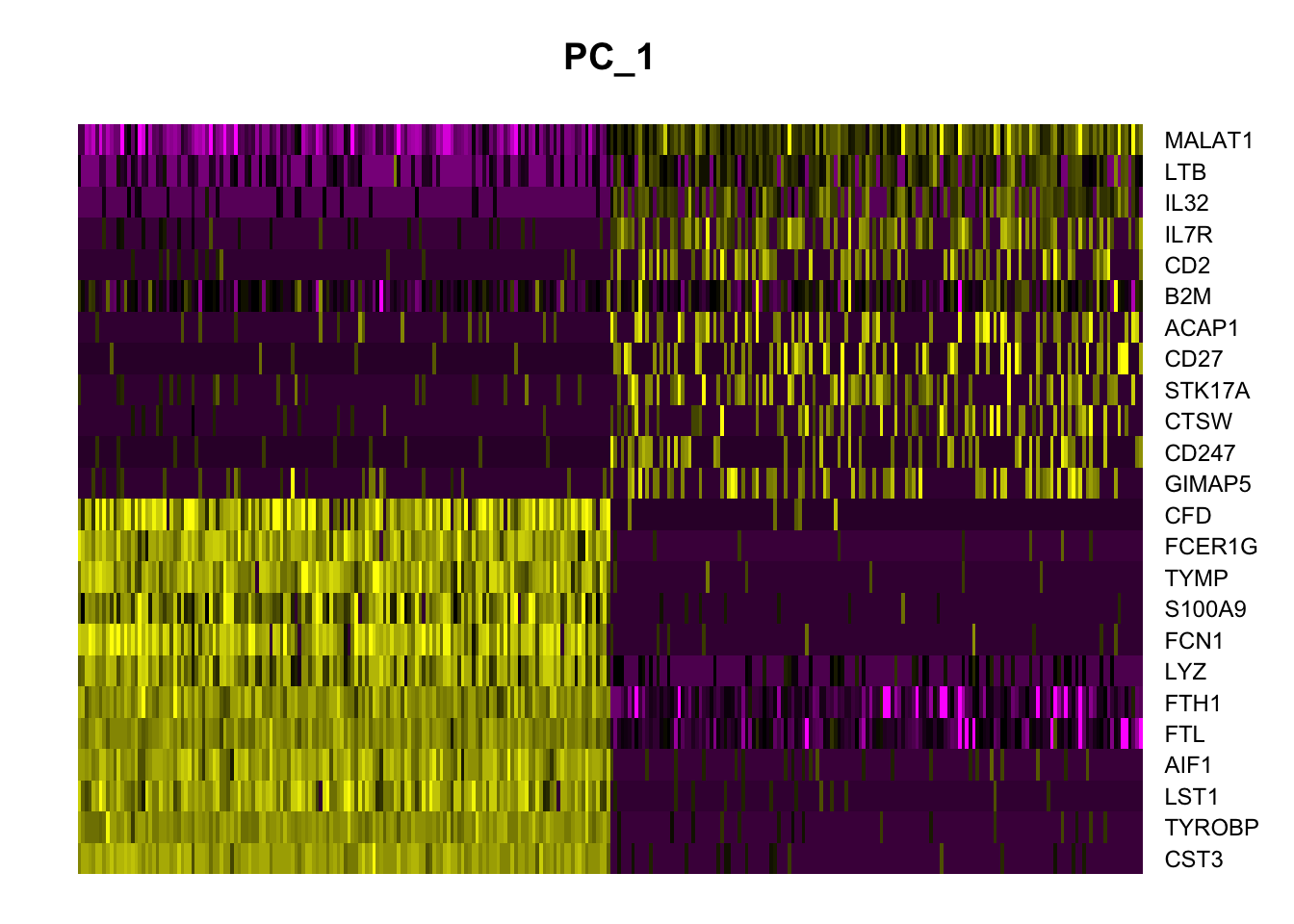
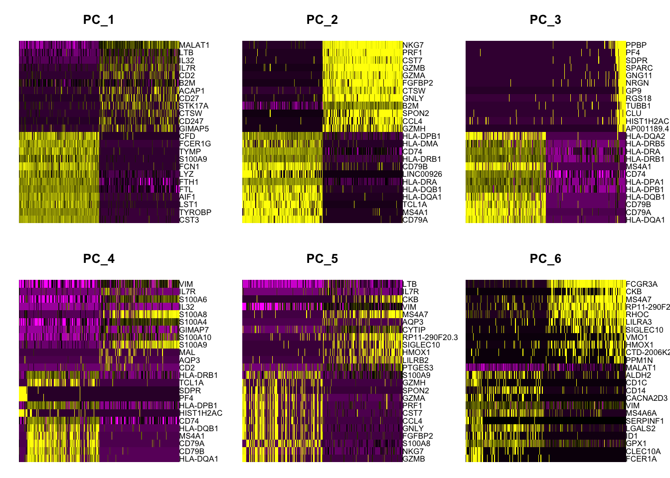
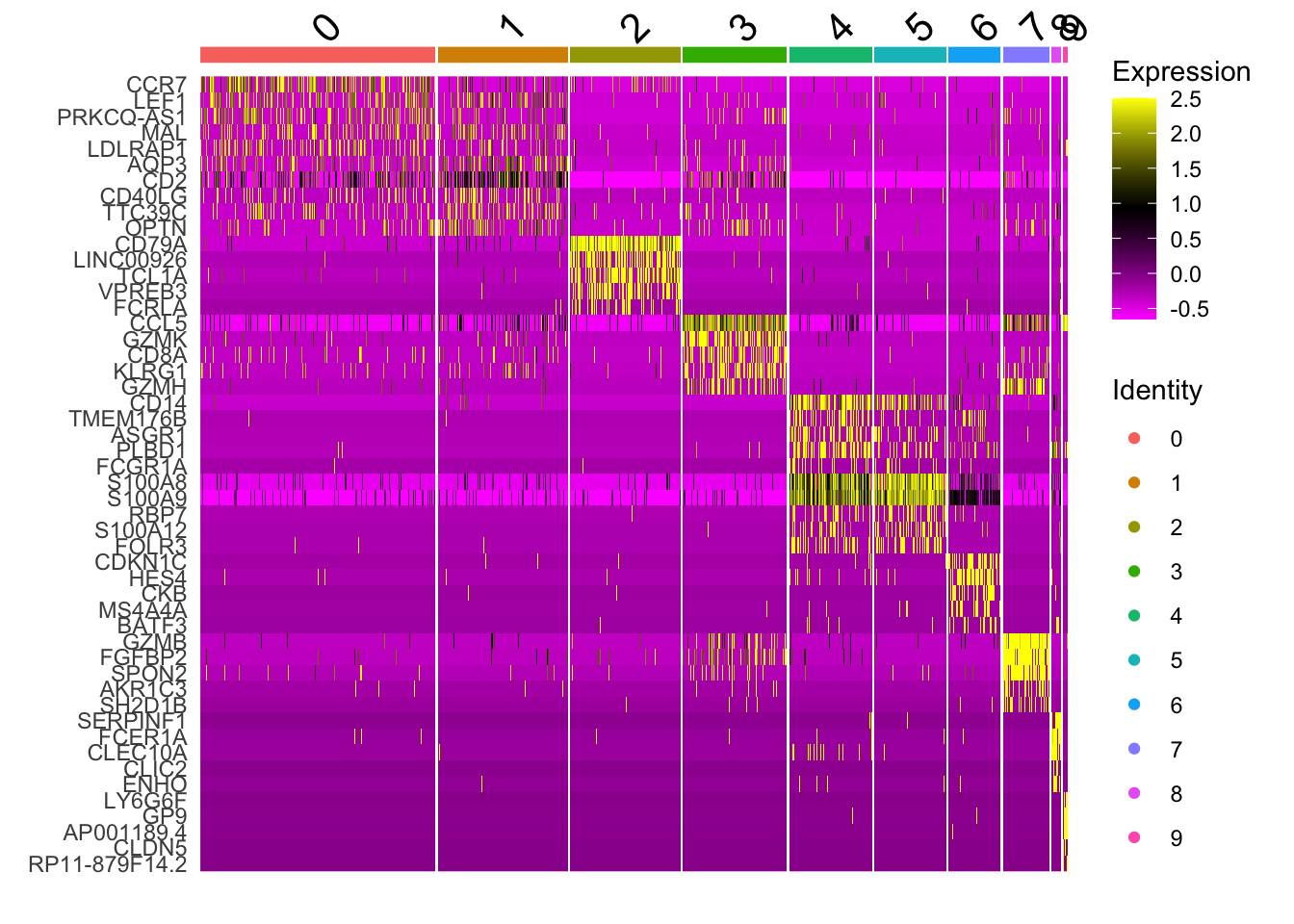
# heatmaps 
# note that 'wt' specifies the variable to use for ordering 
# we get the best markers in terms of size effect
pbmc.markers %>%
    group_by(cluster) %>%
    top_n(n = 5, wt = avg_log2FC) -> top_n

head(top_n,10)

# A tibble: 10 × 7
# Groups:   cluster [2]
      p_val avg_log2FC pct.1 pct.2 p_val_adj cluster gene     
      <dbl>      <dbl> <dbl> <dbl>     <dbl> <fct>   <chr>    
 1 8.18e-99       2.61 0.452 0.098  1.12e-94 0       CCR7     
 2 3.88e-65       2.33 0.358 0.091  5.31e-61 0       LEF1     
 3 9.12e-53       2.11 0.343 0.102  1.25e-48 0       PRKCQ-AS1
 4 2.57e-45       2.19 0.281 0.077  3.52e-41 0       MAL      
 5 5.94e-35       2.43 0.253 0.079  8.15e-31 0       LDLRAP1  
 6 7.64e-61       2.19 0.451 0.116  1.05e-56 1       AQP3     
 7 3.78e-51       1.65 0.658 0.257  5.19e-47 1       CD2      
 8 3.74e-32       1.88 0.273 0.074  5.12e-28 1       CD40LG   
 9 1.11e-29       1.47 0.315 0.101  1.52e-25 1       TTC39C   
10 4.70e-24       1.56 0.313 0.112  6.45e-20 1       OPTN     

# heat map shows that cluster 1 and 2 are not easily distiguished
# by just a few genes others are 
DoHeatmap(pbmc, features = top_n$gene)

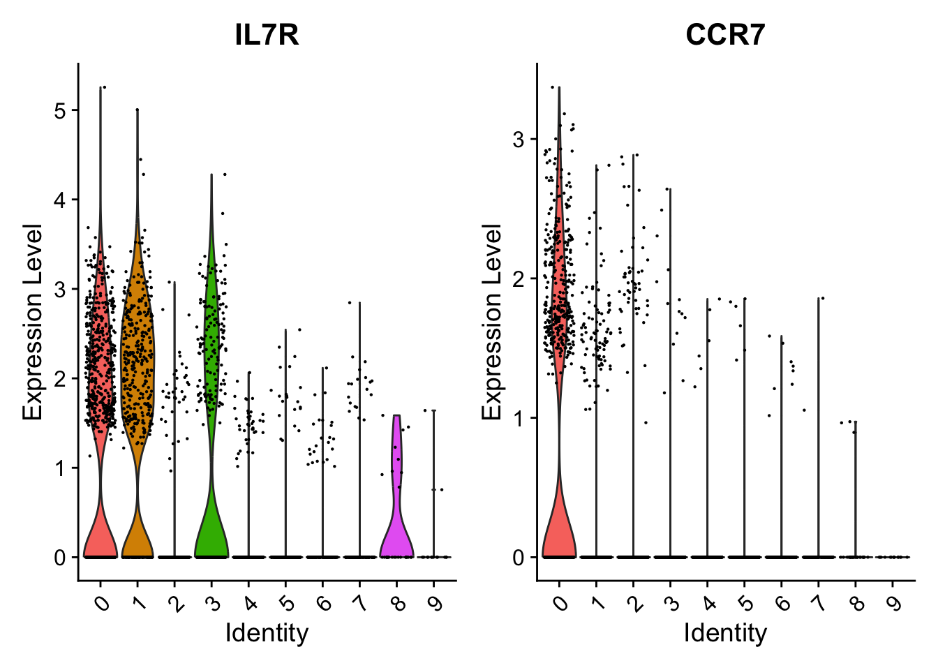
# + NoLegend()

# consider the canonical cluster 0 markers
# "IL7R" is not particularly good marker for cluster 0 
VlnPlot(pbmc, features = c("IL7R", "CCR7"))

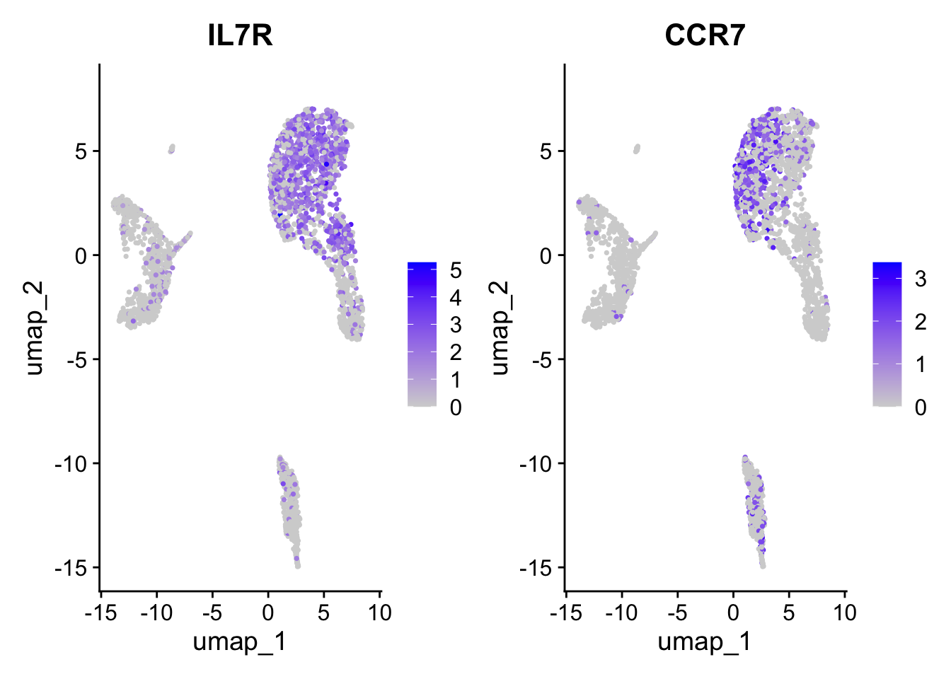
FeaturePlot(pbmc, features = c("IL7R", "CCR7"))

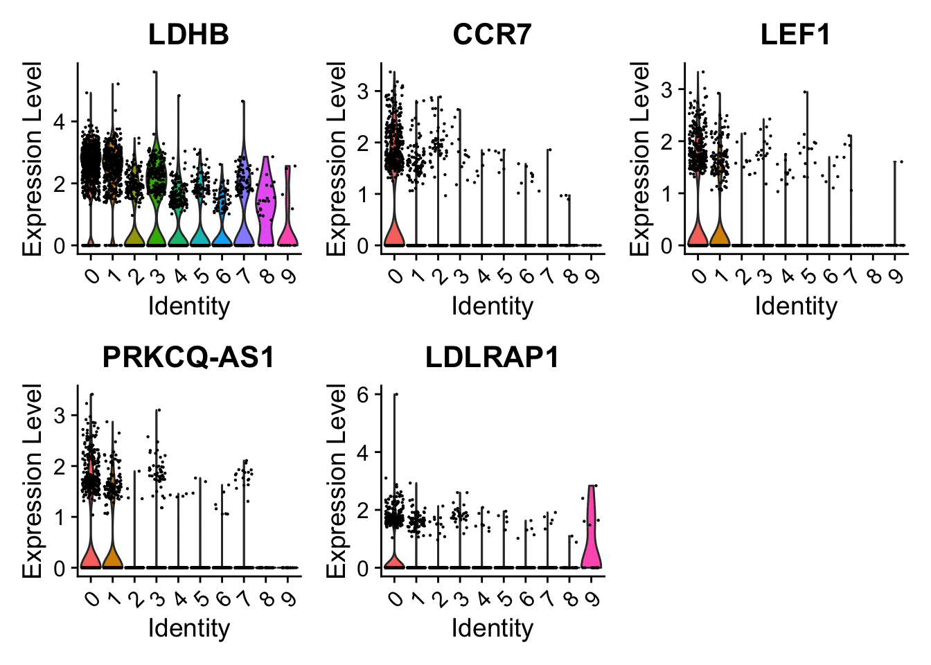
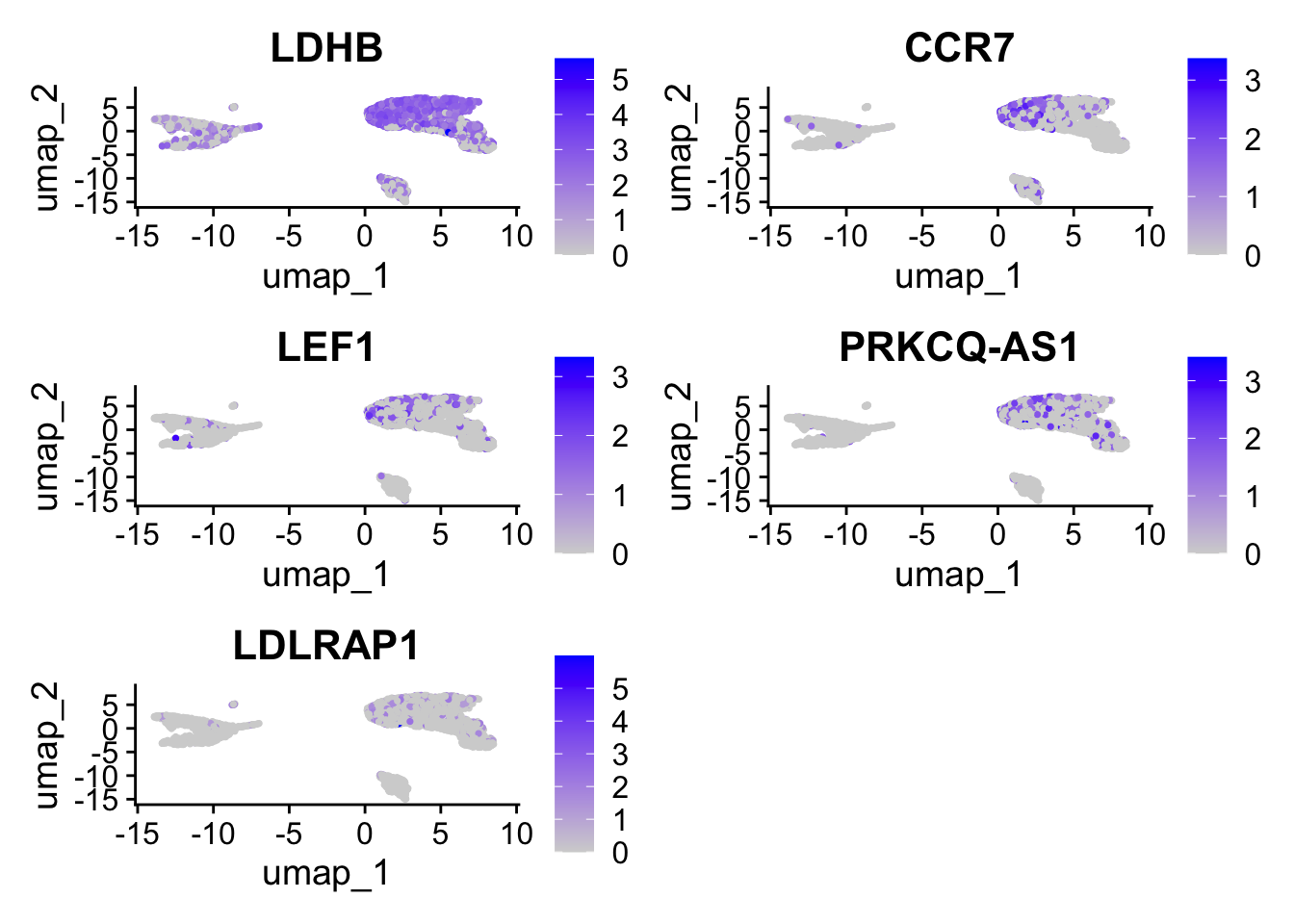
# Try the top 5
# Seems like there are some better markers than IL7R e.g.s LEF1 and PRKCQ-AS1
VlnPlot(pbmc, features = c("LDHB", "CCR7","LEF1","PRKCQ-AS1","LDLRAP1"))

FeaturePlot(pbmc, features = c("LDHB", "CCR7","LEF1","PRKCQ-AS1","LDLRAP1"))

Compare results

• With reference to Example #1 we are just changing the number of PCs used in clustering, tSNE and UMAP
• Using < 10 PCs doesn’t make sense obviously (with reference to the ElbowPlot of variance by PC number) but running a series of increasing n PCs is interesting
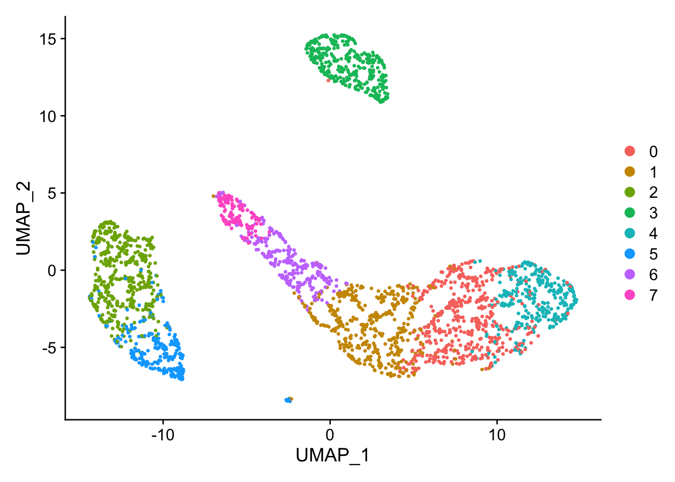
• Here is what happens when 2 instead of 10 PCs are used:

2 Principal Components (Seurat v3)

• …and when 3 instead of 10 PCs are used:

• …and when 5 instead of 10 PCs are used:

5 Principal Components (Seurat v3)

• …and when 7 (n_pcs_chosen should be set to 7, see below) instead of 10 PCs are used:

# just to be sure, echo this number
n_pcs_chosen

[1] 7

# which Seurat?
packageVersion("Seurat")

[1] '5.0.0'

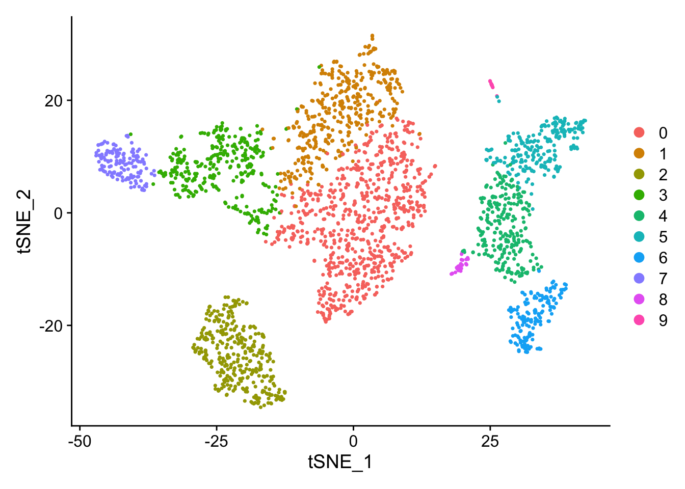
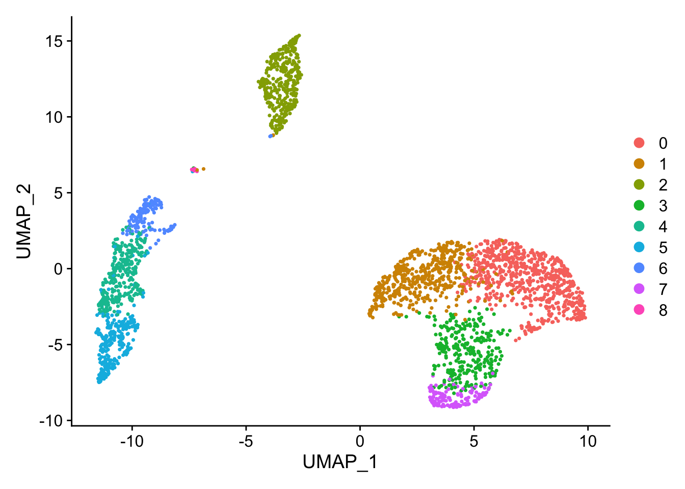
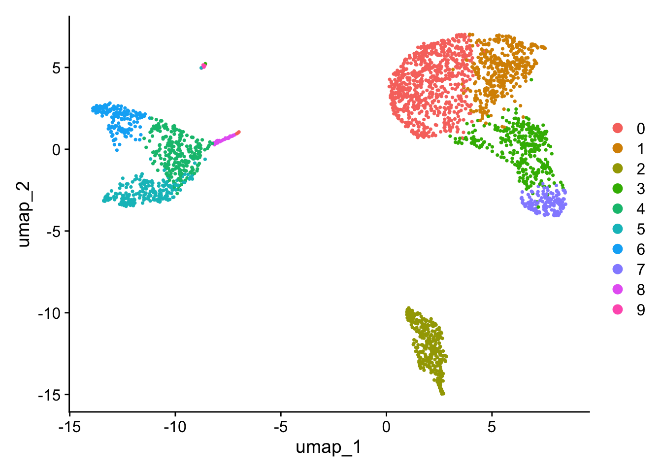
# the unlabelled clusters
DimPlot(pbmc, reduction = "umap")

• Compare with 10 below…

---

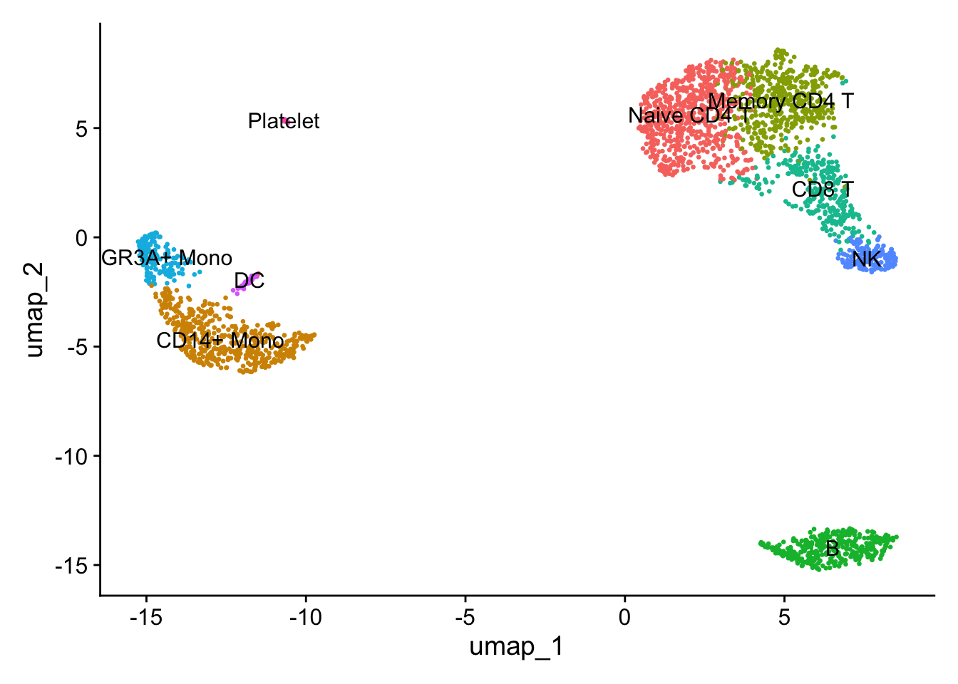
The default labelled UMAP clusters for comparison from Example #1 used 10 PCs (Seurat 5)

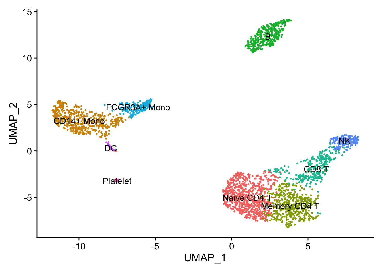
The default labelled UMAP clusters for comparison from Example #1 used 10 PCs (Seurat 3)

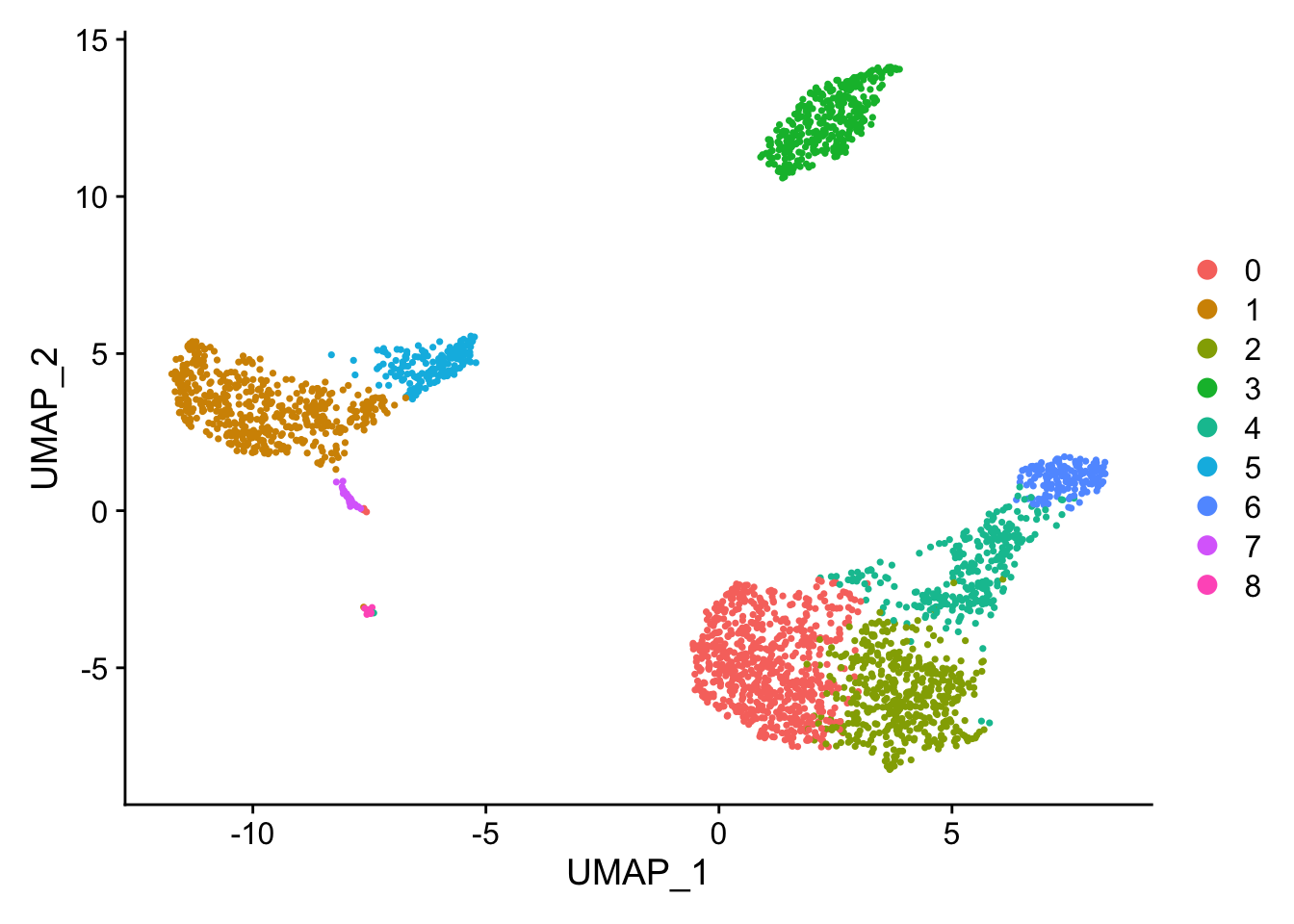
The default unlabelled UMAP clusters for comparison from Example #1 used 10 PCs (Seurat 3)

---

# save final 
file_path <- paste0("./seurat_object_checkpoints/pbmc_sw1",
                    EGN,"_final.rds")
saveRDS_overwrite(file_path)
# Done. See yah :)