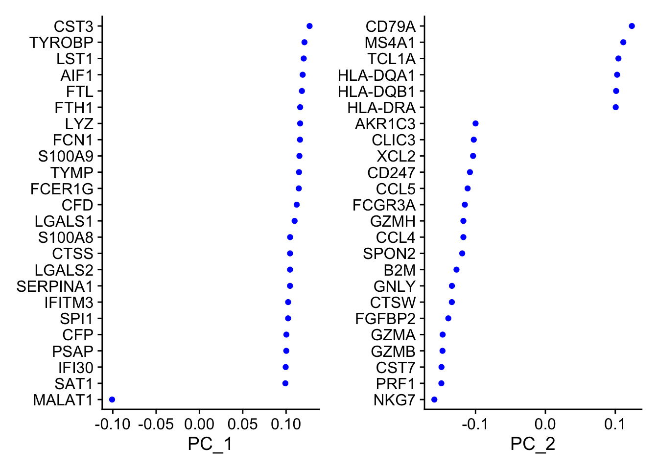
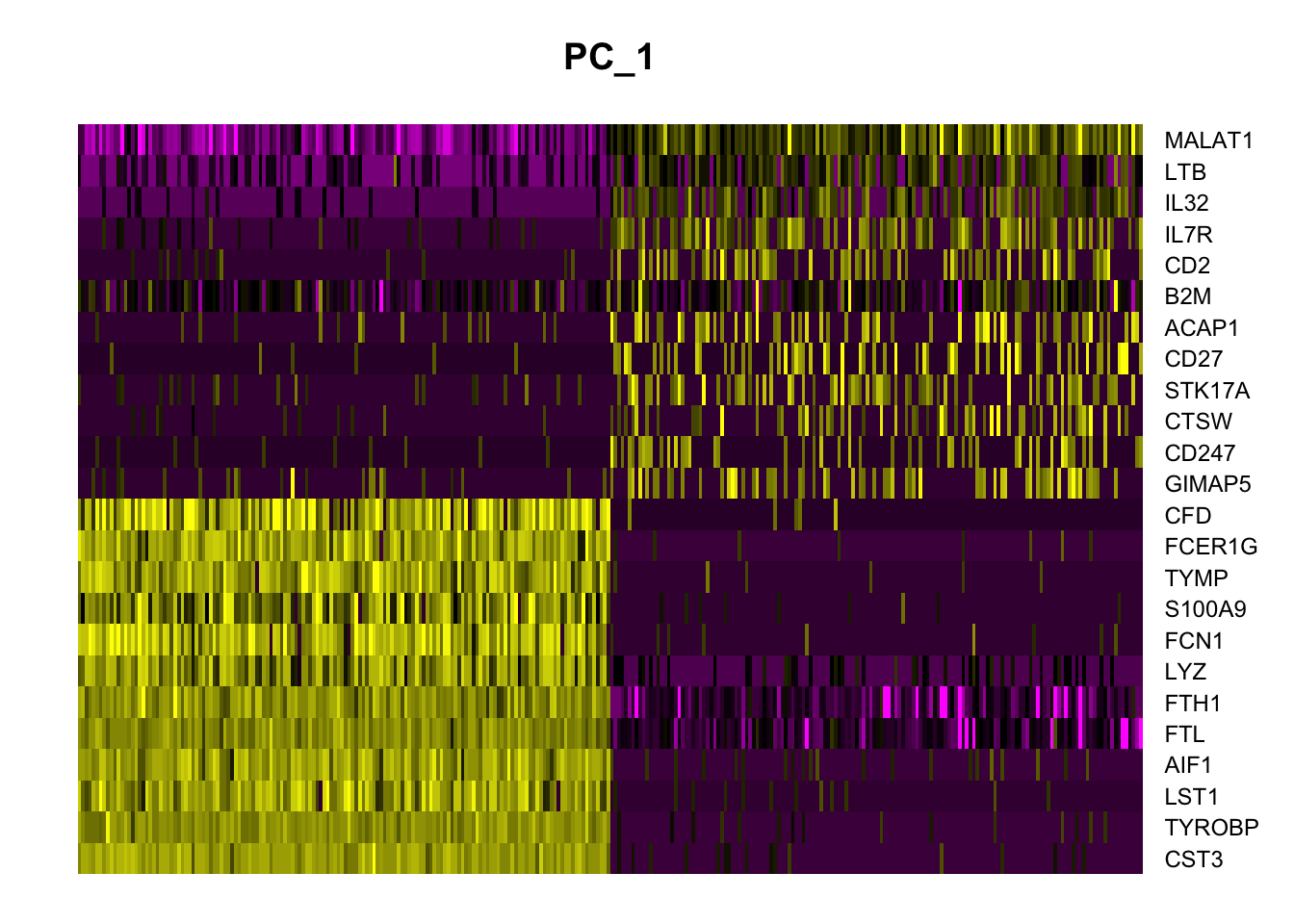
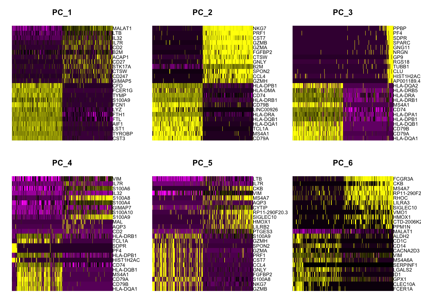
Example #1

Overview

A version of the pbmc3k tutorial from the Satija Lab, together with my own notes, code changes and extensions. The tutorial was re-coded in RStudio as Quarto project, ran on a laptop and published to my github. The focus is on software and data understanding whilst producing the same results. In following example(s), I plan to adjust some parameters to look at the stability of the result with respect to these.

• Study pbmc3k

  • Peripheral Blood Mononuclear Cells (PBMC)

  • 10X Genomics

  • 2,700 single cells

  • sequenced on Illumina NextSeq 500

Background

• Highly Parallel Genome-wide Expression Profiling of Individual Cells Using Nanoliter Droplets

  • Cell, 2015

  • Drop-Seq barcoding schematic

    • primer bead, sequence domains

      • |— PCR —| — cell barcode —| — UMI — | — polyT₂₇ — |

      • UMI: Unique Molecular IDs region

  • Paired end reads

ChangeLog

• These pages were originally developed based on the Seurat v3 vignette and now part updated to Seurat v5
• Some smaller issues need addressing

Includes

Environment Load and Check

• this code section is packaged as an include for reuse across all examples
• it uses the HTML details tag directly to wrap code blocks and output as drop-down sections

Show Environment

library(patchwork)
library(dplyr)

Attaching package: 'dplyr'

The following objects are masked from 'package:stats':

    filter, lag

The following objects are masked from 'package:base':

    intersect, setdiff, setequal, union

library(Seurat)

Loading required package: SeuratObject

Loading required package: sp

'SeuratObject' was built under R 4.3.0 but the current version is
4.3.2; it is recomended that you reinstall 'SeuratObject' as the ABI
for R may have changed

Attaching package: 'SeuratObject'

The following object is masked from 'package:base':

    intersect

• Is there a typo in the message above? Application Programming Interface, API != ABI

• Rolling back to R 4.3.0 was not possible with the current version of Seurat

  • the indication was that Seurat requires a version of base Matrix that is not present in R 4.3.0

# which Seurat?
packageVersion("Seurat")

[1] '5.0.0'

# which R?
version[['version.string']]

[1] "R version 4.3.2 (2023-10-31)"

# presto was installed 
# For a (much!) faster implementation of the 
# Wilcoxon Rank Sum Test
packageVersion('presto')

[1] '1.0.0'

# check python is available via reticulate
import sys
print(sys.version.split(" ")[0])

3.12.0

# shell check
python3 -V

Python 3.12.0

# shell check
quarto -v

1.4.489

Functions

Show Functions

# Useful for code development.
# Save the object at a point and reload it into the R console 
# i.e. for developing alternative reports 
# without having to run the pipeline right from the start
# which can be slow
#
# NB: Files produced by saveRDS (or serialized to a file connection) 
# are not suitable as an interchange format between machines
# 
# For that use hdf5 or transfer data and code to reproduce the result 

saveRDS_overwrite <- function(file_path) {
  if (file.exists(file_path)) {
    file.remove(file_path)
  } 
  saveRDS(pbmc, file = file_path)
}

Data and Config

# Define a constant by convention to identify this example
# To be used as part of filenames when saving objects
# Example Number
EGN <- '_Eg1'

# Data downloaded into git repo 
#   29 MB for barcodes, genes and matrix files 
# NB: these data are already filtered for barcodes within data
# unfiltered would include all possible barcodes 
# (all synthesized barcodes or all theoretical possibilites given
# a certain n of synthesis cycles? would need to delve into bead synthesis here)
data_dir <- "./filtered_gene_bc_matrices/hg19/"
list.files(path = data_dir)

[1] "barcodes.tsv" "genes.tsv"    "matrix.mtx"  

Independent look at data files

# indepenedant look at files to be grounded..
# TSVs
genes_tsv <- read.csv(paste0(data_dir, "genes.tsv"), sep = "\t", header = FALSE)
paste0("n genes: ",nrow(genes_tsv), ". Some rows...")

[1] "n genes: 32738. Some rows..."

head(genes_tsv)

               V1           V2
1 ENSG00000243485   MIR1302-10
2 ENSG00000237613      FAM138A
3 ENSG00000186092        OR4F5
4 ENSG00000238009 RP11-34P13.7
5 ENSG00000239945 RP11-34P13.8
6 ENSG00000237683   AL627309.1

rm(genes_tsv)

barcode_tsv <- read.csv(paste0(data_dir, "barcodes.tsv"), sep = "\t", header = FALSE)
paste0("n cell barcodes: ", nrow(barcode_tsv), ". Some rows...")

[1] "n cell barcodes: 2700. Some rows..."

head(barcode_tsv)

                V1
1 AAACATACAACCAC-1
2 AAACATTGAGCTAC-1
3 AAACATTGATCAGC-1
4 AAACCGTGCTTCCG-1
5 AAACCGTGTATGCG-1
6 AAACGCACTGGTAC-1

rm(barcode_tsv)

# Sample of matrix 
# line 3 is n genes, n cells (barcodes), n lines of data  
# line >3 gene
# gene_id barcode_id, umi_count
readLines(paste0(data_dir, "matrix.mtx"),10)

 [1] "%%MatrixMarket matrix coordinate real general"
 [2] "%"                                            
 [3] "32738 2700 2286884"                           
 [4] "32709 1 4"                                    
 [5] "32707 1 1"                                    
 [6] "32706 1 10"                                   
 [7] "32704 1 1"                                    
 [8] "32703 1 5"                                    
 [9] "32702 1 6"                                    
[10] "32700 1 10"                                   

# we can see sparsity from these numbers
(1 - (2286884 / (32738 * 2700))) * 100

[1] 97.41281

# Sparse Matrix is a "dgTMatrix"
sparse_m <- Matrix::readMM(paste0(data_dir, "matrix.mtx"))
#class(sparse_m)
n_row_genes <- nrow(sparse_m)
n_col_cells <- ncol(sparse_m)
sparsity <- round( sum(sparse_m == 0) / length(sparse_m)  * 100,2)
dgTMatrix_summary <- paste0("n_row_genes: ", n_row_genes, 
                            ", n_col_cells: ", n_col_cells, 
                            ", sparsity: ", sparsity, " %")
dgTMatrix_summary

[1] "n_row_genes: 32738, n_col_cells: 2700, sparsity: 97.41 %"

rm(sparse_m)

Import Data

# creates dgCMatrix of all 3 files content
pbmc.data <- Read10X(data.dir = data_dir)
# class(pbmc.data)

# Seurat object with the raw (non-normalized data).

# Keep genes expressed in at least min.cells
# Include cells where at least min.features are detected
pbmc <- CreateSeuratObject(counts = pbmc.data, 
                           project = "pbmc3k", 
                           min.cells = 3, 
                           min.features = 200)

Warning: Feature names cannot have underscores ('_'), replacing with dashes
('-')

# Seurat object has reduced number of features (genes)
# and possiblly samples (cells) with harsher paremeters
# min.cells = 50, min.features = 400
pbmc

An object of class Seurat 
13714 features across 2700 samples within 1 assay 
Active assay: RNA (13714 features, 0 variable features)
 1 layer present: counts

Pre-processing

Blockquote:

Seurat allows you to easily explore QC metrics and filter cells based on any user-defined criteria. A few QC metrics commonly used by the community include

• The number of unique genes detected in each cell.

  • Low-quality cells or empty droplets will often have very few genes

  • Cell doublets or multiplets may exhibit an aberrantly high gene count

• Similarly, the total number of molecules detected within a cell (correlates strongly with unique genes)

• The percentage of reads that map to the mitochondrial genome

  • Low-quality / dying cells often exhibit extensive mitochondrial contamination

  • We calculate mitochondrial QC metrics with the PercentageFeatureSet() function, which calculates the percentage of counts originating from a set of features

  • We use the set of all genes starting with MT- as a set of mitochondrial genes

Meta data stash, calculations and basis for filtering

# Stashing meta data
head(pbmc@meta.data, 5)

                 orig.ident nCount_RNA nFeature_RNA
AAACATACAACCAC-1     pbmc3k       2419          779
AAACATTGAGCTAC-1     pbmc3k       4903         1352
AAACATTGATCAGC-1     pbmc3k       3147         1129
AAACCGTGCTTCCG-1     pbmc3k       2639          960
AAACCGTGTATGCG-1     pbmc3k        980          521

# The [[ operator can add columns to object metadata. 
# In this case the % mitochondrial DNA based on syntax of gene naming
# 
pbmc[["percent.mt"]] <- PercentageFeatureSet(pbmc, pattern = "^MT-")

head(pbmc@meta.data, 5)

                 orig.ident nCount_RNA nFeature_RNA percent.mt
AAACATACAACCAC-1     pbmc3k       2419          779  3.0177759
AAACATTGAGCTAC-1     pbmc3k       4903         1352  3.7935958
AAACATTGATCAGC-1     pbmc3k       3147         1129  0.8897363
AAACCGTGCTTCCG-1     pbmc3k       2639          960  1.7430845
AAACCGTGTATGCG-1     pbmc3k        980          521  1.2244898

The MT- genes from genes.csv from a bash shell grep. Sure there is a way to get the same from Seurat object.

# bash grep
grep '\tMT-' ./filtered_gene_bc_matrices/hg19/genes.tsv 

ENSG00000198888 MT-ND1
ENSG00000198763 MT-ND2
ENSG00000198804 MT-CO1
ENSG00000198712 MT-CO2
ENSG00000228253 MT-ATP8
ENSG00000198899 MT-ATP6
ENSG00000198938 MT-CO3
ENSG00000198840 MT-ND3
ENSG00000212907 MT-ND4L
ENSG00000198886 MT-ND4
ENSG00000198786 MT-ND5
ENSG00000198695 MT-ND6
ENSG00000198727 MT-CYB

# Visualize QC metrics as a violin plot
VlnPlot(pbmc, features = c("nFeature_RNA", "nCount_RNA", "percent.mt"),
        ncol = 3)

Warning: Default search for "data" layer in "RNA" assay yielded no results;
utilizing "counts" layer instead.

# FeatureScatter is typically used to visualize feature-feature relationships 
# but can be used for anything calculated by the object, 
# i.e. columns in object metadata, PC scores etc.

plot1 <- FeatureScatter(pbmc, feature1 = "nCount_RNA", feature2 = "percent.mt")
plot2 <- FeatureScatter(pbmc, feature1 = "nCount_RNA", feature2 = "nFeature_RNA")
plot1 + plot2

Filtering

Some “exceptions” are dealt with at this stage

• A high ratio of mitochondrial DNA:nuclear DNA is typical of a dead or broken cell

• Multiple cells per drop is atypical but they can be picked up by high number of RNA counts

• Empties are drops without intact cells but produce signal due to background RNA molecules from lyzed cells: they are filtered by having low gene (feature) count but that was already done in this case when the data was imported (see earlier)

• There can be other issues e.g. barcode synthesis errors. Need to fix barcode/remove cell.

• This filtering is at least kingdom specific - think of plant cells and chloroplast RNA, guard cells and endoreduplication….and rapidly dividing cultures of yeast and microbial cells that at the population level partly 2n

# apply filters and overwrite the object!
pbmc <- subset(pbmc, subset = nFeature_RNA > 200 & 
                 nFeature_RNA < 2500 & percent.mt < 5)

# what was the point of storing meta data?!
# 
# It's OK, this meta-data is retained

head(pbmc@meta.data, 5)

                 orig.ident nCount_RNA nFeature_RNA percent.mt
AAACATACAACCAC-1     pbmc3k       2419          779  3.0177759
AAACATTGAGCTAC-1     pbmc3k       4903         1352  3.7935958
AAACATTGATCAGC-1     pbmc3k       3147         1129  0.8897363
AAACCGTGCTTCCG-1     pbmc3k       2639          960  1.7430845
AAACCGTGTATGCG-1     pbmc3k        980          521  1.2244898

# And we can see clearly the effect of filtering
plot1 <- FeatureScatter(pbmc, feature1 = "nCount_RNA", feature2 = "percent.mt")
plot2 <- FeatureScatter(pbmc, feature1 = "nCount_RNA", feature2 = "nFeature_RNA")
plot1 + plot2

Remember nFeature_RNA is the number of detected genes and the nCount_RNA is the total counts per drop (after filtering that should now be per single cell though in the case the one outlier point makes me wonder….seems like ~2000 features is the upper range….).

Another thought in passing: presumably alternative splice forms are mapped to the same gene as standard practice. Would like to look for an example of where splice forms are treated as separate entities which should be in principle possible.

Normalization

After removing unwanted cells from the data-set, the next step is to normalize the data. By default, we employ a global-scaling normalization method “LogNormalize” that normalizes the feature expression measurements for each cell by the total expression, multiplies this by a scale factor (10,000 by default), and log-transforms the result. Normalized values are stored in pbmc[["RNA"]]@data.

# 
pbmc <- NormalizeData(pbmc, normalization.method = "LogNormalize", 
                      scale.factor = 10000)

Normalizing layer: counts

# Show a small sample of data
# Again, it's a sparse matrix 
# class(pbmc[["RNA"]]@data)
# Seurat version 3
# str(pbmc[["RNA"]]@data)

# Seurat version 5
str(pbmc[["RNA"]]$data)

Formal class 'dgCMatrix' [package "Matrix"] with 6 slots
  ..@ i       : int [1:2238732] 29 73 80 148 163 184 186 227 229 230 ...
  ..@ p       : int [1:2639] 0 779 2131 3260 4220 4741 5522 6304 7094 7626 ...
  ..@ Dim     : int [1:2] 13714 2638
  ..@ Dimnames:List of 2
  .. ..$ : chr [1:13714] "AL627309.1" "AP006222.2" "RP11-206L10.2" "RP11-206L10.9" ...
  .. ..$ : chr [1:2638] "AAACATACAACCAC-1" "AAACATTGAGCTAC-1" "AAACATTGATCAGC-1" "AAACCGTGCTTCCG-1" ...
  ..@ x       : num [1:2238732] 1.64 1.64 2.23 1.64 1.64 ...
  ..@ factors : list()

# Seurat version 3
# 10 rows, 3 columns
# pbmc[["RNA"]]@data[10:20,1:3]

# Seurat version 5
pbmc[["RNA"]]$data[10:20,1:3]

11 x 3 sparse Matrix of class "dgCMatrix"
             AAACATACAACCAC-1 AAACATTGAGCTAC-1 AAACATTGATCAGC-1
HES4                        .         .                .       
RP11-54O7.11                .         .                .       
ISG15                       .         .                1.429744
AGRN                        .         .                .       
C1orf159                    .         .                .       
TNFRSF18                    .         1.625141         .       
TNFRSF4                     .         .                .       
SDF4                        .         .                1.429744
B3GALT6                     .         .                .       
FAM132A                     .         .                .       
UBE2J2                      .         .                .       

Highly Variable Features

We next calculate a subset of features that exhibit high cell-to-cell variation in the dataset (i.e, they are highly expressed in some cells, and lowly expressed in others). We and others have found that focusing on these genes in downstream analysis helps to highlight biological signal in single-cell datasets.

Our procedure in Seurat is described in detail here, and improves on previous versions by directly modeling the mean-variance relationship inherent in single-cell data, and is implemented in the FindVariableFeatures() function. By default, we return 2,000 features per dataset. These will be used in downstream analysis, like PCA.

pbmc <- FindVariableFeatures(pbmc, selection.method = "vst", nfeatures = 2000)

Finding variable features for layer counts

# vst: First, fits a line to the relationship of log(variance) and log(mean) using local 
# polynomial regression (loess). Then standardizes the feature values using the observed mean # and expected variance (given by the fitted line). Feature variance is then calculated on 
# the standardized values after clipping to a maximum (see clip.max parameter).
# 
# Other selection methods available mean.var.plot (mvp) and dispersion (disp)
#

# Identify a number (n_top) of highly variable genes from 
n_top <- 15
top_v_genes <- head(VariableFeatures(pbmc), n_top)
top_v_genes

 [1] "PPBP"    "LYZ"     "S100A9"  "IGLL5"   "GNLY"    "FTL"     "PF4"    
 [8] "FTH1"    "GNG11"   "S100A8"  "FCER1A"  "HLA-DRA" "CD74"    "CLU"    
[15] "NKG7"   

# plot variable features with and without labels
plot1 <- VariableFeaturePlot(pbmc)
plot2 <- LabelPoints(plot = plot1, points = top_v_genes, repel = TRUE)

When using repel, set xnudge and ynudge to 0 for optimal results

# no need to view this, plot2 is better
#plot1
plot2 

Warning: Transformation introduced infinite values in continuous x-axis

Data Scaling

Normally i do a mean 0, standard dev 1 … but the method used here is more sophisticated.

Next, we apply a linear transformation (‘scaling’) that is a standard pre-processing step prior to dimensional reduction techniques like PCA. The ScaleData() function:

• Shifts the expression of each gene, so that the mean expression across cells is 0

• Scales the expression of each gene, so that the variance across cells is 1

  • This step gives equal weight in downstream analyses, so that highly-expressed genes do not dominate

• The results of this are stored in pbmc[["RNA"]]@scale.data

all.genes <- rownames(pbmc)
pbmc <- ScaleData(pbmc, features = all.genes)

Centering and scaling data matrix

And there is a faster way…

Scaling is an essential step in the Seurat workflow, but only on genes that will be used as input to PCA. Therefore, the default in ScaleData() is only to perform scaling on the previously identified variable features (2,000 by default). To do this, omit the features argument in the previous function call, i.e.

pbmc <- ScaleData(pbmc)

Your PCA and clustering results will be unaffected. However, Seurat heatmaps (produced as shown below with DoHeatmap()) require genes in the heatmap to be scaled, to make sure highly-expressed genes don’t dominate the heatmap. To make sure we don’t leave any genes out of the heatmap later, we are scaling all genes in this tutorial.

This following section refers to the paper Normalization and variance stabilization of single-cell RNA-seq data using regularized negative binomial regression Christoph Hafemeister & Rahul Satija (2019). I have this in paper notes as the method to deal with cell cycle genes. Interesting would be circadian cycle - I came across experimental data before that hadn’t considered this aspect in the experimental design!!

How can I remove unwanted sources of variation, as in Seurat v2?

In Seurat v2 we also use the ScaleData() function to remove unwanted sources of variation from a single-cell dataset. For example, we could ‘regress out’ heterogeneity associated with (for example) cell cycle stage, or mitochondrial contamination. These features are still supported in ScaleData() in Seurat v3, i.e.:

pbmc <- ScaleData(pbmc, vars.to.regress = "percent.mt")

However, particularly for advanced users who would like to use this functionality, we strongly recommend the use of our new normalization workflow, SCTransform(). The method is described in our paper, with a separate vignette using Seurat v3 here. As with ScaleData(), the function SCTransform() also includes a vars.to.regress parameter.

Linear Dimension Reduction

Run PCA with the scaled data values

• by dafault a subset of genes corresponding to the variability calculation done previously in this workflow, although the subset is configurable at this stage

# example of changing feature subset for calculation
pbmc <- RunPCA(pbmc, features = VariableFeatures(object = pbmc))
# but for now we just run with the default....

# verbose is by dafault TRUE 
# it spits out a number of PCs (ndims.print = 1:5) 
# and genes (features) contributing to each PC (nfeatures.print = 30) 
pbmc <- RunPCA(pbmc, verbose = FALSE)
# we could adjust those arguments or do the same more directly
# by just jumping into the object's data structure
#
# the number to print 
n_features <- 8
print(pbmc[["pca"]], dims = 1:4, nfeatures = n_features)

PC_ 1 
Positive:  CST3, TYROBP, LST1, AIF1, FTL, FTH1, LYZ, FCN1 
Negative:  MALAT1, LTB, IL32, IL7R, CD2, B2M, ACAP1, CD27 
PC_ 2 
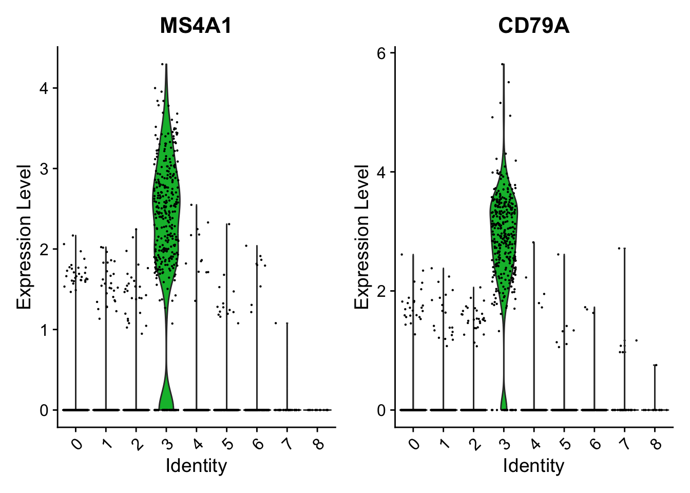
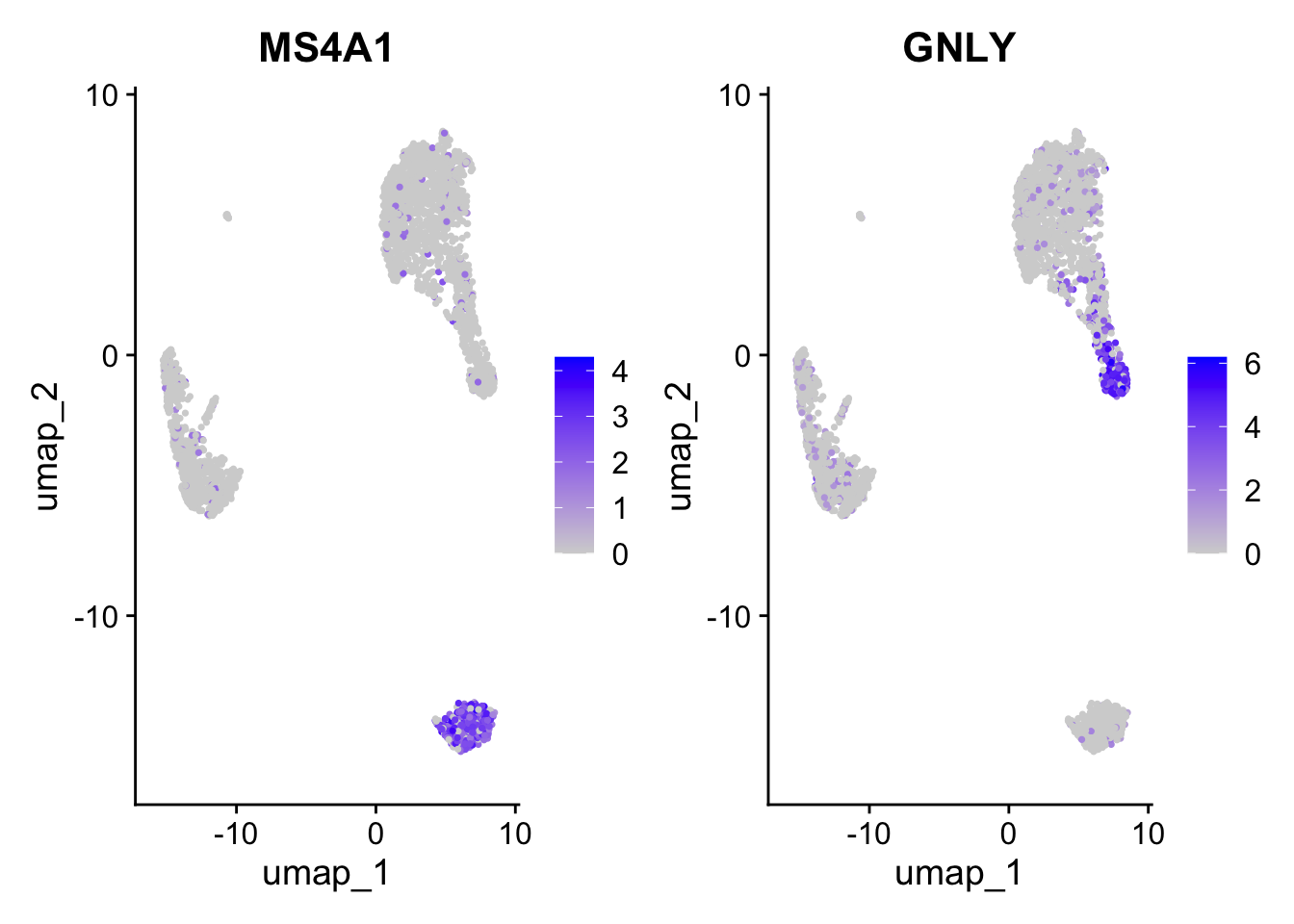
Positive:  CD79A, MS4A1, TCL1A, HLA-DQA1, HLA-DQB1, HLA-DRA, LINC00926, CD79B 
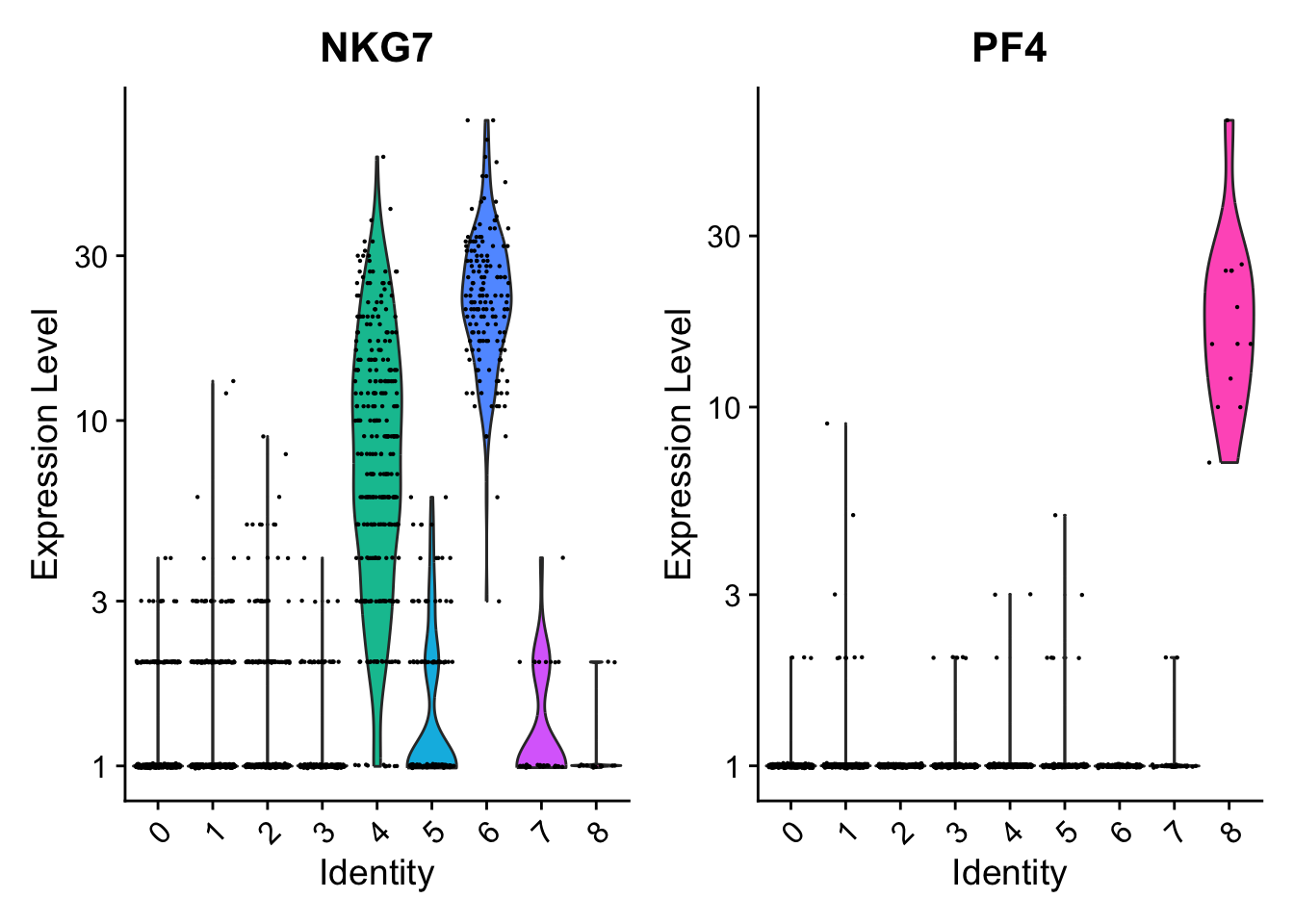
Negative:  NKG7, PRF1, CST7, GZMB, GZMA, FGFBP2, CTSW, GNLY 
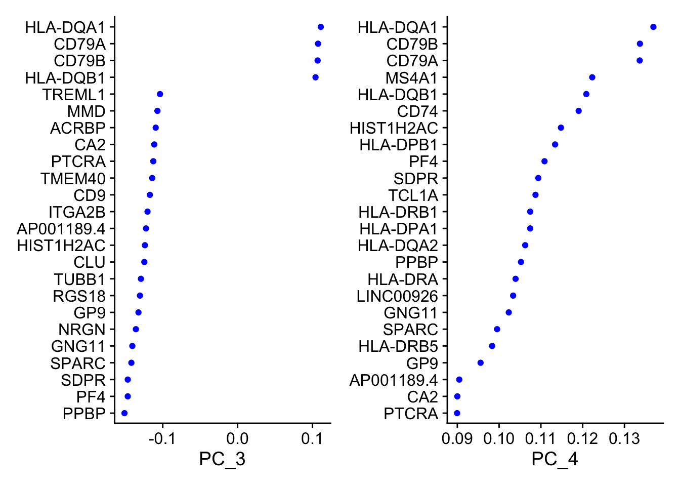
PC_ 3 
Positive:  HLA-DQA1, CD79A, CD79B, HLA-DQB1, HLA-DPB1, HLA-DPA1, CD74, MS4A1 
Negative:  PPBP, PF4, SDPR, SPARC, GNG11, NRGN, GP9, RGS18 
PC_ 4 
Positive:  HLA-DQA1, CD79B, CD79A, MS4A1, HLA-DQB1, CD74, HIST1H2AC, HLA-DPB1 
Negative:  VIM, IL7R, S100A6, IL32, S100A8, S100A4, GIMAP7, S100A10 

Look at the loadings matrix (V) and scores(U)

V

# Loadings
# 
# best to use n * n_features, otherwise we can get plots that are biased to 
# either +ve or -ve contributions preseumably because nfeatures takes from a 
# ranked list disregarding sign
#
# e.g. see loadings of PC_4, no negatives plotted using n_features = 8
#
n_mulitplier = 3
VizDimLoadings(pbmc, dims = 1:2, 
               reduction = "pca", 
               nfeatures = n_features * n_mulitplier)

VizDimLoadings(pbmc, dims = 3:4, 
               reduction = "pca", 
               nfeatures = n_features * n_mulitplier)

U

# Dimplot has lots of options
DimPlot(pbmc, reduction = "pca",  dims = c(1, 2))

DimPlot(pbmc, reduction = "pca",  dims = c(2, 3))

Heatmaps

Blockquote:

In particular DimHeatmap() allows for easy exploration of the primary sources of heterogeneity in a dataset, and can be useful when trying to decide which PCs to include for further downstream analyses. Both cells and features are ordered according to their PCA scores. Setting cells to a number plots the ‘extreme’ cells on both ends of the spectrum, which dramatically speeds plotting for large datasets. Though clearly a supervised analysis, we find this to be a valuable tool for exploring correlated feature sets.

Just 1

# as in quote above, 
# ordererd cells and genes according to PCA scores 
# 
n_cells <- 300
n_genes <- 24
DimHeatmap(pbmc, dims = 1, cells = n_cells, nfeatures = n_genes, balanced = TRUE)

Many

# balanced
n_PC <- 6
plots <- DimHeatmap(pbmc, dims = 1:n_PC, cells = n_cells, 
             nfeatures = n_genes, balanced = TRUE)

if (0){
  # for later...something not quite right with feature labels
  # unbalanced 
  plots <- DimHeatmap(pbmc, dims = 1:n_PC, cells = n_cells, 
             nfeatures = n_genes, balanced = FALSE)
}

Determine Dimensionality

The traditional way

# how many PCs provide a useable amount of information to distinguish our cells? 
ElbowPlot(pbmc)

The sophisticated way

In Macosko et al, we implemented a resampling test inspired by the JackStraw procedure. We randomly permute a subset of the data (1% by default) and rerun PCA, constructing a ‘null distribution’ of feature scores, and repeat this procedure. We identify ‘significant’ PCs as those who have a strong enrichment of low p-value features.

The JackStrawPlot() function provides a visualization tool for comparing the distribution of p-values for each PC with a uniform distribution (dashed line). ‘Significant’ PCs will show a strong enrichment of features with low p-values (solid curve above the dashed line). In this case it appears that there is a sharp drop-off in significance after the first 10-12 PCs.

n_dims <- 15
# fast
n_reps <- 5
# slow - my laptop is no server
# n_reps <- 100
pbmc <- JackStraw(pbmc, num.replicate = n_reps)
pbmc <- ScoreJackStraw(pbmc, dims = 1:n_dims)
JackStrawPlot(pbmc, dims = 1:n_dims)

Warning: Removed 22880 rows containing missing values (`geom_point()`).

---

JackstrawPlot: 15 dimensions, 100 replicates. This version of the figure was computed in around 10 minutes on laptop. For the sake of speed the previous image was calculated with a small number of replicates.

---

# we can set a variable to specifiy the number of PCs to use
# and later perturb this with iterations to look into the stability of
# the final result

n_pcs_chosen <- 10
#n_pcs_chosen <- 5
#n_pcs_chosen <- 15

Cell Clustering

Blockquote:

Seurat v3 applies a graph-based clustering approach, building upon initial strategies in (Macosko et al). Importantly, the distance metric which drives the clustering analysis (based on previously identified PCs) remains the same. However, our approach to partitioning the cellular distance matrix into clusters has dramatically improved. Our approach was heavily inspired by recent manuscripts which applied graph-based clustering approaches to scRNA-seq data [SNN-Cliq, Xu and Su, Bioinformatics, 2015] and CyTOF data [PhenoGraph, Levine et al., Cell, 2015]. Briefly, these methods embed cells in a graph structure - for example a K-nearest neighbor (KNN) graph, with edges drawn between cells with similar feature expression patterns, and then attempt to partition this graph into highly interconnected ‘quasi-cliques’ or ‘communities’.

As in PhenoGraph, we first construct a KNN graph based on the euclidean distance in PCA space, and refine the edge weights between any two cells based on the shared overlap in their local neighborhoods (Jaccard similarity). This step is performed using the FindNeighbors() function, and takes as input the previously defined dimensionality of the dataset (first 10 PCs).

To cluster the cells, we next apply modularity optimization techniques such as the Louvain algorithm (default) or SLM [SLM, Blondel et al., Journal of Statistical Mechanics], to iteratively group cells together, with the goal of optimizing the standard modularity function. The FindClusters() function implements this procedure, and contains a resolution parameter that sets the ‘granularity’ of the downstream clustering, with increased values leading to a greater number of clusters. We find that setting this parameter between 0.4-1.2 typically returns good results for single-cell datasets of around 3K cells. Optimal resolution often increases for larger datasets. The clusters can be found using the Idents() function.

# create the K-nearest neighbor (KNN) graph of cells
pbmc <- FindNeighbors(pbmc, dims = 1:n_pcs_chosen)

Computing nearest neighbor graph

Computing SNN

# define clusters according to resolution
pbmc <- FindClusters(pbmc, resolution = 0.5)

Modularity Optimizer version 1.3.0 by Ludo Waltman and Nees Jan van Eck

Number of nodes: 2638
Number of edges: 95927

Running Louvain algorithm...
Maximum modularity in 10 random starts: 0.8728
Number of communities: 9
Elapsed time: 0 seconds

# Look at cluster IDs of the first 5 cells
# In this case we have 9 levels (0 - 8)
# The structure is the relation between cell barcode and the cluster (community) 
head(Idents(pbmc), 5)

AAACATACAACCAC-1 AAACATTGAGCTAC-1 AAACATTGATCAGC-1 AAACCGTGCTTCCG-1 
               2                3                2                1 
AAACCGTGTATGCG-1 
               6 
Levels: 0 1 2 3 4 5 6 7 8

# Each cell that survived filtering above is represented 
length(Idents(pbmc))

[1] 2638

pbmc

An object of class Seurat 
13714 features across 2638 samples within 1 assay 
Active assay: RNA (13714 features, 2000 variable features)
 3 layers present: counts, data, scale.data
 1 dimensional reduction calculated: pca

Non-Linear Dimensional Reduction

Blockquote:

Seurat offers several non-linear dimensional reduction techniques, such as tSNE and UMAP, to visualize and explore these datasets. The goal of these algorithms is to learn the underlying manifold of the data in order to place similar cells together in low-dimensional space. Cells within the graph-based clusters determined above should co-localize on these dimension reduction plots. As input to the UMAP and tSNE, we suggest using the same PCs as input to the clustering analysis.

# UMAP
pbmc <- RunUMAP(pbmc, dims = 1:n_pcs_chosen)

Warning: The default method for RunUMAP has changed from calling Python UMAP via reticulate to the R-native UWOT using the cosine metric
To use Python UMAP via reticulate, set umap.method to 'umap-learn' and metric to 'correlation'
This message will be shown once per session

16:24:09 UMAP embedding parameters a = 0.9922 b = 1.112

16:24:09 Read 2638 rows and found 10 numeric columns

16:24:09 Using Annoy for neighbor search, n_neighbors = 30

16:24:09 Building Annoy index with metric = cosine, n_trees = 50

0%   10   20   30   40   50   60   70   80   90   100%

[----|----|----|----|----|----|----|----|----|----|

**************************************************|
16:24:10 Writing NN index file to temp file /var/folders/zp/wn7hdby52ds73hv9g_dxlk380000gn/T//RtmpdHJwEi/file175031e7effa
16:24:10 Searching Annoy index using 1 thread, search_k = 3000
16:24:11 Annoy recall = 100%
16:24:11 Commencing smooth kNN distance calibration using 1 thread with target n_neighbors = 30
16:24:11 Initializing from normalized Laplacian + noise (using RSpectra)
16:24:12 Commencing optimization for 500 epochs, with 105140 positive edges
16:24:17 Optimization finished

DimPlot(pbmc, reduction = "umap")

# tSNE
pbmc <- RunTSNE(pbmc, dims = 1:n_pcs_chosen)
DimPlot(pbmc, reduction = "tsne")

Check-Point The Object

Note that the pmbc can be saved and reloaded with the R base package function

# save the object
file_path <- paste0("./seurat_object_checkpoints/pbmc_sw1",EGN,".rds")
saveRDS_overwrite(file_path)

# NB: Files produced by saveRDS (or serialize to a file connection) 
# are not suitable as an interchange format between machines

# restore the object from disk
pbmc <- readRDS(file_path)

Cluster Biomarkers

Differentially expressed genes between a given cluster and the cell population as a whole or as an alternative, select specific clusters

Blockquote:

Seurat can help you find markers that define clusters via differential expression. By default, it identifies positive and negative markers of a single cluster (specified in ident.1), compared to all other cells. FindAllMarkers() automates this process for all clusters, but you can also test groups of clusters vs. each other, or against all cells.

The min.pct argument requires a feature to be detected at a minimum percentage in either of the two groups of cells, and the thresh.test argument requires a feature to be differentially expressed (on average) by some amount between the two groups. You can set both of these to 0, but with a dramatic increase in time - since this will test a large number of features that are unlikely to be highly discriminatory. As another option to speed up these computations, max.cells.per.ident can be set. This will downsample each identity class to have no more cells than whatever this is set to. While there is generally going to be a loss in power, the speed increases can be significant and the most highly differentially expressed features will likely still rise to the top.

# find all markers of cluster 2
cluster2.markers <- FindMarkers(pbmc, ident.1 = 2, min.pct = 0.25)
head(cluster2.markers, n = 5)

            p_val avg_log2FC pct.1 pct.2    p_val_adj
IL32 2.892340e-90  1.3070772 0.947 0.465 3.966555e-86
LTB  1.060121e-86  1.3312674 0.981 0.643 1.453850e-82
CD3D 8.794641e-71  1.0597620 0.922 0.432 1.206097e-66
IL7R 3.516098e-68  1.4377848 0.750 0.326 4.821977e-64
LDHB 1.642480e-67  0.9911924 0.954 0.614 2.252497e-63

# find all markers distinguishing cluster 5 from clusters 0 and 3
cluster5.markers <- FindMarkers(pbmc, ident.1 = 5, 
                                ident.2 = c(0, 3), min.pct = 0.25)
head(cluster5.markers, n = 5)

                      p_val avg_log2FC pct.1 pct.2     p_val_adj
FCGR3A        8.246578e-205   6.794969 0.975 0.040 1.130936e-200
IFITM3        1.677613e-195   6.192558 0.975 0.049 2.300678e-191
CFD           2.401156e-193   6.015172 0.938 0.038 3.292945e-189
CD68          2.900384e-191   5.530330 0.926 0.035 3.977587e-187
RP11-290F20.3 2.513244e-186   6.297999 0.840 0.017 3.446663e-182

# find markers for every cluster compared to all remaining cells, 
# report only the positive ones
pbmc.markers <- FindAllMarkers(pbmc, only.pos = TRUE, 
                               min.pct = 0.25, logfc.threshold = 0.25)

Calculating cluster 0

Calculating cluster 1

Calculating cluster 2

Calculating cluster 3

Calculating cluster 4

Calculating cluster 5

Calculating cluster 6

Calculating cluster 7

Calculating cluster 8

pbmc.markers %>%
    group_by(cluster) %>%
    slice_max(n = 2, order_by = avg_log2FC)

# A tibble: 18 × 7
# Groups:   cluster [9]
       p_val avg_log2FC pct.1 pct.2 p_val_adj cluster gene         
       <dbl>      <dbl> <dbl> <dbl>     <dbl> <fct>   <chr>        
 1 9.57e- 88       2.40 0.447 0.108 1.31e- 83 0       CCR7         
 2 1.35e- 51       2.14 0.342 0.103 1.86e- 47 0       LEF1         
 3 7.07e-139       7.28 0.299 0.004 9.70e-135 1       FOLR3        
 4 3.38e-121       6.74 0.277 0.006 4.64e-117 1       S100A12      
 5 2.97e- 58       2.09 0.42  0.111 4.07e- 54 2       AQP3         
 6 5.03e- 34       1.87 0.263 0.07  6.90e- 30 2       CD40LG       
 7 2.40e-272       7.38 0.564 0.009 3.29e-268 3       LINC00926    
 8 2.75e-237       7.14 0.488 0.007 3.76e-233 3       VPREB3       
 9 7.25e-165       4.41 0.577 0.055 9.95e-161 4       GZMK         
10 3.27e- 88       3.74 0.419 0.061 4.48e- 84 4       GZMH         
11 8.23e-168       5.88 0.37  0.005 1.13e-163 5       CKB          
12 1.69e-212       5.43 0.506 0.01  2.32e-208 5       CDKN1C       
13 8.10e-179       6.22 0.471 0.013 1.11e-174 6       AKR1C3       
14 5.38e-112       6.07 0.29  0.007 7.38e-108 6       SH2D1B       
15 1.46e-207       8.03 0.5   0.002 2.00e-203 7       SERPINF1     
16 1.48e-220       7.63 0.812 0.011 2.03e-216 7       FCER1A       
17 0              14.4  0.615 0     0         8       LY6G6F       
18 7.32e-222      13.9  0.385 0     1.00e-217 8       RP11-879F14.2

Blockquote:

Seurat has several tests for differential expression which can be set with the test.use parameter (see our DE vignette for details). For example, the ROC test returns the ‘classification power’ for any individual marker (ranging from 0 - random, to 1 - perfect).

cluster0.markers <- FindMarkers(pbmc, ident.1 = 0, 
                                logfc.threshold = 0.25, 
                                test.use = "roc", only.pos = TRUE)

head(cluster0.markers,20)

       myAUC  avg_diff power avg_log2FC pct.1 pct.2
RPS12  0.827 0.5059247 0.654  0.7387061 1.000 0.991
RPS6   0.826 0.4762402 0.652  0.6934523 1.000 0.995
RPS27  0.824 0.5047203 0.648  0.7372604 0.999 0.992
RPL32  0.821 0.4294911 0.642  0.6266075 0.999 0.995
RPS14  0.811 0.4334133 0.622  0.6336957 1.000 0.994
RPS25  0.803 0.5196163 0.606  0.7689940 0.997 0.975
RPL31  0.798 0.5227603 0.596  0.7757544 0.997 0.964
RPL9   0.797 0.5230934 0.594  0.7714338 0.997 0.971
RPL13  0.792 0.3893890 0.584  0.5659877 1.000 0.996
RPL3   0.788 0.4200060 0.576  0.6134175 0.997 0.995
RPS3   0.788 0.4104851 0.576  0.5989384 1.000 0.994
RPS3A  0.787 0.5461948 0.574  0.8010270 0.997 0.975
RPL30  0.785 0.4606356 0.570  0.6806394 1.000 0.980
LDHB   0.784 0.7521034 0.568  1.2060189 0.912 0.592
RPL21  0.783 0.4576652 0.566  0.6709538 0.997 0.991
RPS15A 0.782 0.4417193 0.564  0.6484728 0.997 0.983
RPLP2  0.776 0.4113912 0.552  0.6031631 1.000 0.990
RPS27A 0.770 0.5076242 0.540  0.7454804 0.994 0.967
RPS13  0.769 0.4814302 0.538  0.7159655 0.985 0.962
EEF1A1 0.769 0.3662114 0.538  0.5358999 0.994 0.991

Blockquote:

We include several tools for visualizing marker expression. VlnPlot() (shows expression probability distributions across clusters), and FeaturePlot() (visualizes feature expression on a tSNE or PCA plot) are our most commonly used visualizations. We also suggest exploring RidgePlot(), CellScatter(), and DotPlot() as additional methods to view your dataset.

VlnPlot(pbmc, features = c("MS4A1", "CD79A"))

VlnPlot(pbmc, features = c("NKG7", "PF4"), slot = "counts", log = TRUE)

Warning: The `slot` argument of `VlnPlot()` is deprecated as of Seurat 5.0.0.
ℹ Please use the `layer` argument instead.

# the 3 x 3 grid did not look clear on my laptop
# try by 2 
FeaturePlot(pbmc, features = c("MS4A1", "GNLY"))

FeaturePlot(pbmc, features = c("CD3E", "CD14"))

FeaturePlot(pbmc, features = c("FCER1A", "FCGR3A"))

FeaturePlot(pbmc, features = c("LYZ", "PPBP"))

FeaturePlot(pbmc, features = c("CD8A"))

Blockquote:

DoHeatmap() generates an expression heatmap for given cells and features. In this case, we are plotting the top 20 markers (or all markers if less than 20) for each cluster.

# the default was 10 
# the heatmap is hard to read with so many markers
# would need to produce a larger version with high label resolution 
pbmc.markers %>%
    group_by(cluster) %>%
    top_n(n = 5, wt = avg_log2FC) -> top_n

head(top_n,10)

# A tibble: 10 × 7
# Groups:   cluster [2]
       p_val avg_log2FC pct.1 pct.2 p_val_adj cluster gene     
       <dbl>      <dbl> <dbl> <dbl>     <dbl> <fct>   <chr>    
 1 9.57e- 88       2.40 0.447 0.108 1.31e- 83 0       CCR7     
 2 1.35e- 51       2.14 0.342 0.103 1.86e- 47 0       LEF1     
 3 2.81e- 44       1.53 0.443 0.185 3.85e- 40 0       PIK3IP1  
 4 6.27e- 43       1.99 0.33  0.112 8.60e- 39 0       PRKCQ-AS1
 5 1.34e- 34       1.96 0.268 0.087 1.84e- 30 0       MAL      
 6 0               6.65 0.975 0.121 0         1       S100A8   
 7 0               6.18 0.996 0.215 0         1       S100A9   
 8 1.03e-295       5.98 0.667 0.027 1.42e-291 1       CD14     
 9 7.07e-139       7.28 0.299 0.004 9.70e-135 1       FOLR3    
10 3.38e-121       6.74 0.277 0.006 4.64e-117 1       S100A12  

DoHeatmap(pbmc, features = top_n$gene) + NoLegend()

Cell Type Identity To Clusters

Blockquote:

Fortunately in the case of this data-set, we can use canonical markers to easily match the unbiased clustering to known cell types:

---

Known cell type markers

---

new.cluster.ids <- c("Naive CD4 T", "CD14+ Mono", "Memory CD4 T", 
                     "B", "CD8 T", "FCGR3A+ Mono",
                    "NK", "DC", "Platelet")
names(new.cluster.ids) <- levels(pbmc)
pbmc <- RenameIdents(pbmc, new.cluster.ids)
DimPlot(pbmc, reduction = "umap", label = TRUE, pt.size = 0.5) + NoLegend()

file_path <- paste0("./seurat_object_checkpoints/pbmc_sw1",EGN,"_final.rds")
saveRDS_overwrite(file_path)
# Done. See yah :)